Nov 24, 2023

Fortran 2023 (ISO/IEC 1539-1:2023) has been officially published. This replaces the previous standard (Fortran 2018). In a previous post I listed the updates that are in this release (then called "Fortran 202x"). It will be a while before we have fully-compliant Fortran 2023 compilers. In the latest update to the Intel Fortran Compiler, they have started to add a few minor things.
Fortran is the oldest surviving programming language still in common use. Originally developed in 1957, first standardized in 1966, and continuously updated since that time, Fortran remains at the heart of scientific and high-performance computing.
The next standard (unofficially called Fortran 202y) is also already in work.

See also
- Programming languages: Fortran, ISO, Nov. 17, 2023.
- S. Lionel, Fortran 2023 has been Published!, Nov. 23, 2023.
- John Reid, The new features of Fortran 2023, Mar. 13, 2023.
- J. Williams, The New Features of Fortran 202x, Mar 27, 2022.
- Fortran: High-performance parallel programming language
Oct 12, 2022

Image created with the assistance of NightCafe Creator.
Historically, large general-purpose libraries have formed the core of the Fortran scientific ecosystem (e.g., SLATEC, or the various PACKS). Unfortunately, as I have mentioned here before, these libraries were written in FORTRAN 77 (or earlier) and remained unmodified for decades. The amazing algorithms continued within them imprisoned in a terrible format that nobody wants to deal with anymore. At the time they were written, they were state of the art. Now they are relics of the past, a reminder of what might have been if they had continued to be maintained and Fortran had continued to remain the primary scientific and technical programming language.
Over the last few years, I've managed to build up a pretty good set of modern Fortran libraries for technical computing. Some are original, but a lot of them include modernized code from the libraries written decades ago. The codes still work great (polyroots-fortran contains a modernized version of a routine written 50 years ago), but they just needed a little bit of cleanup and polish to be presentable to modern programmers as something other than ancient legacy to be tolerated but not well maintained (which is how Fortran is treated in the SciPy ecosystem).
Here is the list:
| Catagory |
Library |
Description |
Release |
| Interpolation |
bspline-fortran |
1D-6D B-Spline Interpolation |
 |
| Interpolation |
regridpack |
1D-4D linear and cubic interpolation |
 |
| Interpolation |
finterp |
1D-6D Linear Interpolation |
 |
| Interpolation |
PCHIP |
Piecewise Cubic Hermite Interpolation Package |
 |
| Plotting |
pyplot-fortran |
Make plots from Fortran using Matplotlib |
 |
| File I/O |
json-fortran |
Read and write JSON files |
 |
| File I/O |
fortran-csv-module |
Read and write CSV Files |
 |
| Optimization |
slsqp |
SLSQP Optimizer |
 |
| Optimization |
fmin |
Derivative free 1D function minimizer |
 |
| Optimization |
pikaia |
Pikaia Genetic Algorithm |
 |
| Optimization |
simulated-annealing |
Simulated Annealing Algorithm |
 |
| One Dimensional Root-Finding |
roots-fortran |
Roots of continuous scalar functions of a single real variable, using derivative-free methods |
 |
| Polynomial Roots |
polyroots-fortran |
Root finding for real and complex polynomial equations |
 |
| Nonlinear equations |
nlesolver-fortran |
Nonlinear Equation Solver |
 |
| Ordinary Differential Equations |
dop853 |
An explicit Runge-Kutta method of order 8(5,3) |
 |
| Ordinary Differential Equations |
ddeabm |
DDEABM Adams-Bashforth algorithm |
 |
| Numerical Differentiation |
NumDiff |
Numerical differentiation with finite differences |
 |
| Numerical integration |
quadpack |
Modernized QUADPACK Library for 1D numerical quadrature |
 |
| Numerical integration |
quadrature-fortran |
1D-6D Adaptive Gaussian Quadrature |
 |
| Random numbers |
mersenne-twister-fortran |
Mersenne Twister pseudorandom number generator |
 |
| Astrodynamics |
Fortran-Astrodynamics-Toolkit |
Modern Fortran Library for Astrodynamics |
 |
| Astrodynamics |
astro-fortran |
Standard models used in fundamental astronomy |
 |
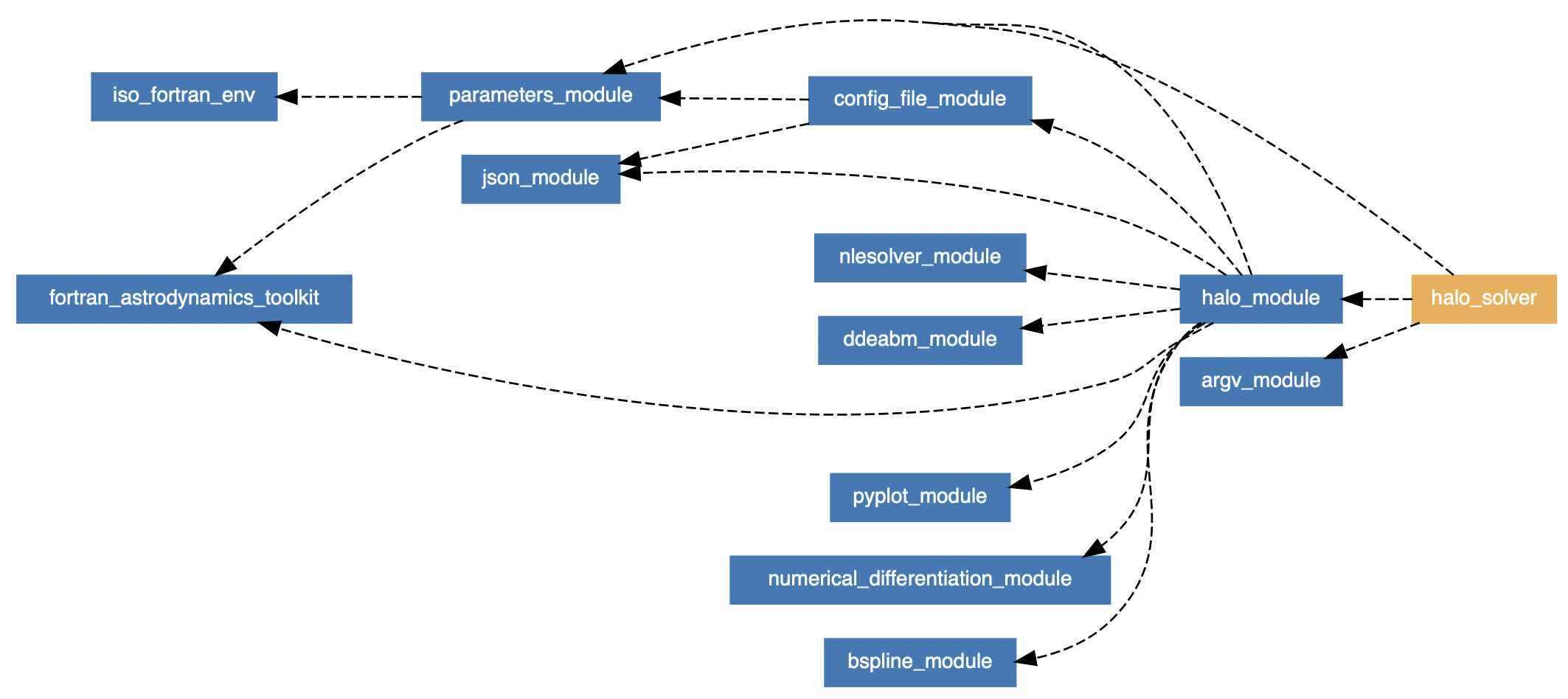
Example of module dependencies in a Fortran application. This is for the Halo solver.
All of these libraries satisfy my requirements for being part of a modern Fortran scientific ecosystem:
- All are written in a modern Fortran style (free-form, modules, no obsolete constructs such as gotos or common blocks, etc.) All legacy code has been modernized.
- They are all usable with the Fortran Package Manager. A couple of previous posts here and here show how easy it is to do this with a one-line addition to your FPM manifest file.
- The real kind (single, double, or quad precision) is selectable via a preprocessor directive.
- All libraries are available in git repositories on GitHub and contributions are welcome. Every commit is unit tested using GitHub CI.
- All the sourcecode is documented online using FORD.
- All have permissive licenses (e.g., BSD-3) so you can use them however you want.
Fortran has many advantages for scientific computing. It's fast, standard, statically typed, compiled, stable, has a nice array syntax, and includes object oriented programming and native parallelism. It is great for technical and numerical codes that need to run fast and are intended to be used for decades. The libraries listed above will not stop working in a few years. An extremely complicated Fortran application can be recompiled with just a Fortran compiler. You cannot say the same for anything written in the Python scientific ecosystem, which is a Frankenstein hybrid of a scripting language hacked together with a pile of C/C++/Fortran libraries compiled by somebody else. Good luck trying to run Python you write now 20 years from now (or trying to run something written 20 years ago). Fortran is a simple and stable foundation upon which to build our scientific software, Python is not. Having readily available modern libraries along with recent improvements in the Fortran tooling and ecosystem should only serve to make Fortran more appealing in this area.
See also
Jul 31, 2022
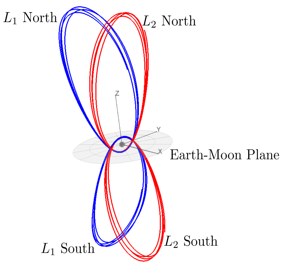
Some Earth-Moon NRHOs. From Williams et al, 2017.
I have mentioned the Circular Restricted Three-Body Problem (CR3BP) here a couple of times. Another type of periodic CR3BP orbit is the "near rectilinear" halo orbit (NRHO). These orbits are just the continuation of the family of "normal" halo orbits until they get very close to the secondary body [1]. Like all halo orbits, there are "northern" and "southern" families (see image above). NASA chose a lunar L2 NRHO (southern family, which spends more time over the lunar South pole) as the destination orbit for the Deep Space Gateway [2].
The CAPSTONE mission [3] successfully launched on June 28, 2022, and is currently en route to the Gateway NRHO. [4-5]
Computing an NRHO
A basic NRHO in the CR3BP can be computed just like a "normal" halo orbit. (see this and this earlier post). In Reference [2] we described methods for generating long-duration NRHOs in a realistic force model. The procedure involves a multiple shooting method using the CR3BP solution as an initial guess replicated for multiple revs of the orbit. Then a simple nonlinear solver is used to impose state and time continuity for the full orbit.
All we need to start the process is an initial guess. Appendix A.1 in Reference [6] lists a table of CR3BP Earth-Moon L2 halo orbits. An example NRHO from this table is shown here:
| Parameter |
Value |
| \(l^{*}\) |
384400.0 |
| \(t^{*}\) |
375190.25852 |
| Jacobi constant |
3.0411 |
| period |
1.5872714606 |
| \(x_0\) |
1.0277926091 |
| \(z_0\) |
-0.1858044184 |
| \(\dot y_0\) |
-0.1154896637 |
In this table, the three state parameters (\(x_0\), \(z_0\), and \(\dot y_0\)) are given in the canonical normalized CR3BP system, with respect to the Earth-Moon barycenter. The distance and time normalization factors (\(l^{*}\) and \(t^{*}\)) can be used to convert them into normal distance and time units (km and sec).
The process is fairly straightforward, and is demonstrated in a new tool, which I call Halo. It is written in Modern Fortran.
The Halo tool uses the initial CR3BP state to generate a long-duration orbit in the real ephemeris model.
Halo doesn't use the CR3BP equations of motion, since we will be integrating in the real system, using the actual ephemeris of the Earth and Moon, and so we use the real units. See Reference [7] for some further details about an earlier version of this code.
Halo is built upon a number of open source Fortran libraries, and the main components of the tool are:
- General astrodynamics routines, including: ephemeris of the Sun, Earth, and Moon, a spherical harmonic lunar gravity model, state transformations, etc. These are all provided by the Fortran Astrodynamics Toolkit.
- A numerical integration method. I'm using DDEABM, which is an Adams method. I like this method, which has a long heritage and seems to have a good balance of speed and accuracy for these kinds of astrodynamics problems.
- A way to compute derivatives, which are needed by the solver for the Jacobian. For this problem, finite-difference numerical derivatives are good enough, so I'm using my NumDiff library. Since the problem ends up being quite sparse, we can use the NumDiff options to quickly compute the Jacobian matrix by taking into account the sparsity pattern.
- A nonlinear numerical solver. I'm using my nlsolver-fortran library. The problem being solved is "underdetermined", meaning there are more free variables than there are constraints. Nlsolver-Fortran can solve these problems just fine using a basic Newton-type minimum norm method. In astrodynamics, you will usually see this type of method called a "differential corrector".
Halo makes use of the amazing Fortran Package Manager (FPM) for dependency management and compilation. In the fpm.toml manifest file, all we have to do is specify the dependencies like so:
[dependencies]
fortran-astrodynamics-toolkit = { git = "https://github.com/jacobwilliams/Fortran-Astrodynamics-Toolkit", tag = "0.4" }
NumDiff = { git = "https://github.com/jacobwilliams/NumDiff", tag = "1.5.1" }
ddeabm = { git = "https://github.com/jacobwilliams/ddeabm", tag = "3.0.0" }
json-fortran = { git = "https://github.com/jacobwilliams/json-fortran", tag = "8.2.5" }
bspline-fortran = { git = "https://github.com/jacobwilliams/bspline-fortran", tag = "6.1.0" }
pyplot-fortran = { git = "https://github.com/jacobwilliams/pyplot-fortran", tag = "3.2.0" }
fortran-search-and-sort = { git = "https://github.com/jacobwilliams/fortran-search-and-sort", tag = "1.0.0" }
fortran-csv-module = { git = "https://github.com/jacobwilliams/fortran-csv-module", tag = "1.3.0" }
nlesolver-fortran = { git = "https://github.com/jacobwilliams/nlesolver-fortran", tag = "1.0.0" }
argv-fortran = { git = "https://github.com/jacobwilliams/argv-fortran", tag = "1.0.0" }
FPM will download the specified versions of everything and build the tool with a single command like so:
fpm build --profile release
This is really a game changer for Fortran. Before FPM, poor Fortran users had no package manager at all. A common anti-pattern was to manually download code from somewhere like Netlib and then manually add the files to your repo and manually edit your makefiles to incorporate it into your compile process. This is literally what SciPy has done, and now they have forks of all their Fortran code that just lives inside the SciPy monorepo, with no way to distribute it upstream to the original library source, or downstream to other Fortran codes that might want to use it. FPM makes it all just effortless to specify dependencies (and update the version numbers if the upstream code changes) and finally allows and encourages Fortran users to develop a modern system of interdependent libraries with sane and modern version control practices.
Example
Using the initial guess from the table above, we can use Halo to compute a ballistic NRHO for 50 revs (about 344 days for this example) in the real ephemeris model. The 50 rev problem has 1407 control variables and 1200 equality constraints. Convergence takes about 31 seconds (6 iterations of the solver) on my M1 MacBook Pro, complied using the Intel Fortran compiler:
| Iteration number |
norm2(Constraint violation vector) |
| 1 |
0.2936000870578949 |
| 2 |
0.1554308242228055 |
| 3 |
0.0611200979653433 |
| 4 |
0.0052758762761737 |
| 5 |
0.0000031933098398 |
| 6 |
0.0000000035186120 |
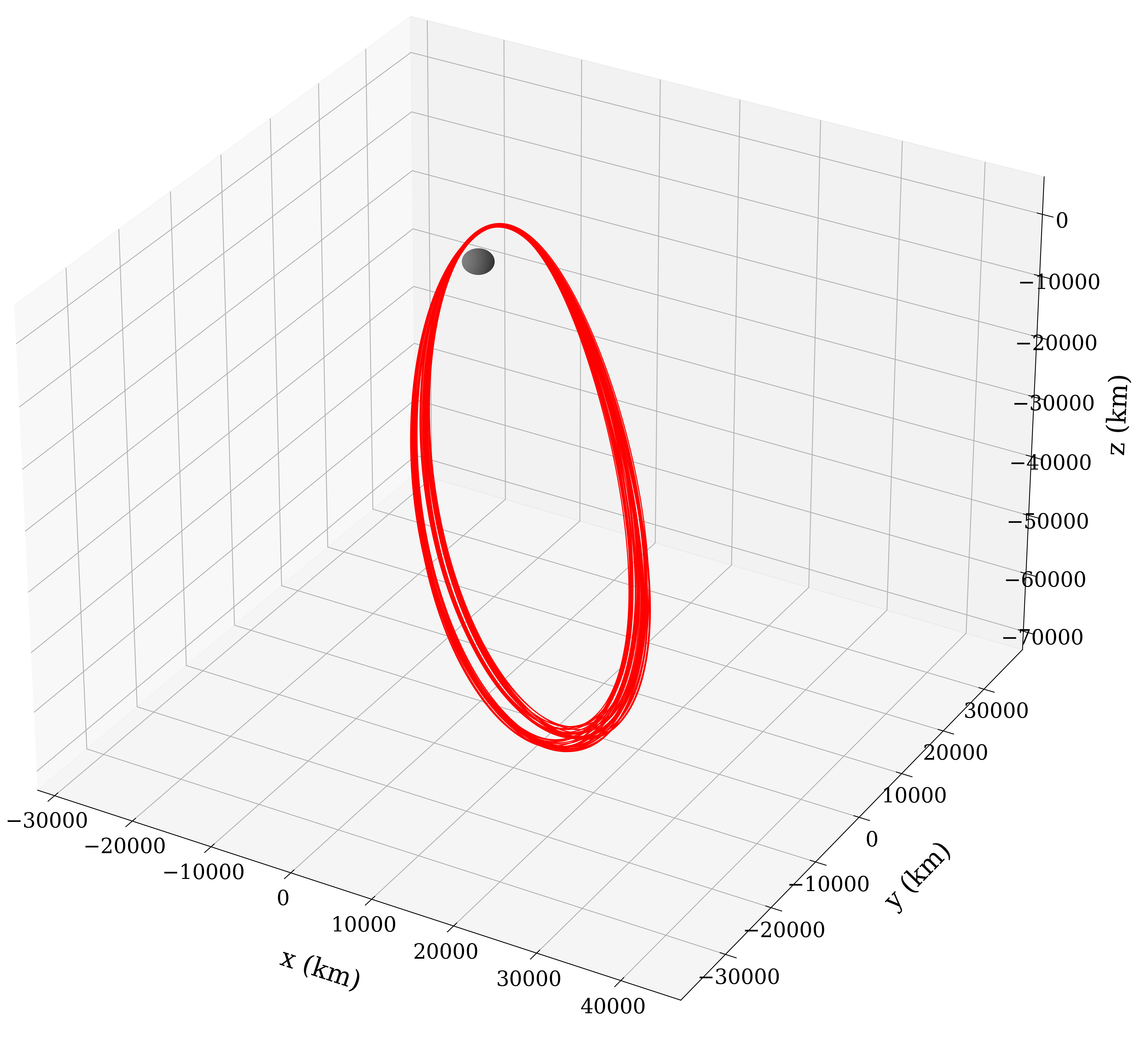
50 Rev NRHO Solution. Visualized here in the Moon-centered Earth-Moon rotating frame.
There's no parallelization currently being used here, so there are some opportunities to speed it up even more.
In Reference [2] we also show how the above procedure can be used to kick off a "receding horizon" approach to compute even longer duration NRHOs that include very small correction burns. This is the process that was used to generate the Gateway orbit [4-5], and the Halo program could be updated to do that as well. But that is a post for another time.
See also
- K. C. Howell & J. V. Breakwell, "Almost rectilinear halo orbits", Celestial mechanics volume 32, pages 29--52 (1984)
- J. Williams, D. E. Lee, R. J. Whitley, K. A. Bokelmann, D. C. Davis, and C. F. Berry. "Targeting cislunar near rectilinear halo orbits for human space exploration", AAS 17-267
- What is CAPSTONE?, NASA, Apr 29, 2022
- D. E. Lee, "Gateway Destination Orbit Model: A Continuous 15 Year NRHO Reference Trajectory", August 20, 2019
- D. E. Lee, R. J. Whitley and C. Acton, "Sample Deep Space Gateway Orbit, NAIF Planetary Data System Navigation Node", NASA Jet Propulsion Laboratory, July 2018.
- E. M. Z. Spreen, "Trajectory Design and Targeting For Applications to the Exploration Program in Cislunar Space", PhD Dissertation, Purdue University, 2021
- J. Williams, R. D. Falck, and I. B. Beekman, "Application of Modern Fortran to Spacecraft Trajectory Design and Optimization", 2018 Space Flight Mechanics Meeting, 8–12 January 2018, AIAA 2018-145.
Jun 19, 2022

NightCafe AI generated image for "old computers"
The classic Fortran routines r1mach (for single precision real numbers), d1mach (for double precision real numbers), and i1mach (for integers) were originally written in the mid-1970s for the purpose of returning basic machine or operating system dependent constants in order to provide portability. Typically, these routines had a bunch of commented out DATA statements, and the user was required to uncomment out the ones for their specific machine. The original versions included constants for the following systems:
Over the years, various versions of these routines have been created:
In the Fortran 90 versions, the original routines were modified to use various intrinsic functions available in Fortran 90. However, some hard-coded values remained in i1mach. With the advent of more recent standards, it is now possible to provide modern and completely portable versions which are described below. Starting with the Fortran 90 versions, the following changes were made:
- The routines are now in a module. We declare two module parameters which will be used in the routines:
integer, parameter :: sp = kind(1.0)    ! single precision kind
integer, parameter :: dp = kind(1.0d0)  ! double precision kind
Of course, putting them in a module means that they are not quite drop-in replacements for the old routines. If you want to use this module with legacy code, you'd have to update your code to add a use statement. But that's the way it goes. Nobody should be writing Fortran anymore that isn't in a module, so I'm not going to encourage that.
-
The comment strings have been updated to Ford-style. I find the old SLATEC comment block style extremely cluttered. Various cosmetic changes were also made (e.g., changing the old .GE. to >=, etc.)
-
All three routines were made pure. The error stop construct was used for the out of bounds input condition (Fortran 2008 allows error stop in pure procedures).
-
New intrinsic constants available in the Fortran 2008 standard were employed (see below).
The new routines can be found on GitHub. They are shown below without the comment blocks.
The new routines
The new d1mach routine is:
D1MACH
  pure real(dp) function d1mach(i)

    integer, intent(in) :: i

    real(dp), parameter :: x = 1.0_dp
    real(dp), parameter :: b = real(radix(x), dp)

    select case (i)
    case (1); d1mach = b**(minexponent(x) - 1) ! the smallest positive magnitude.
    case (2); d1mach = huge(x)                 ! the largest magnitude.
    case (3); d1mach = b**(-digits(x))         ! the smallest relative spacing.
    case (4); d1mach = b**(1 - digits(x))      ! the largest relative spacing.
    case (5); d1mach = log10(b)
    case default
        error stop 'Error in d1mach - i out of bounds'
    end select

  end function d1mach
This is mostly just a reformatting of the Fortran 90 routine. We make x and b parameters, and use error stop for the error condition rather than this monstrosity:
          WRITE (*, FMT = 9000)
 9000     FORMAT ('1ERROR    1 IN D1MACH - I OUT OF BOUNDS')
          STOP
R1MACH
The updated R1MACH is similar, except the real values are real(sp) (default real, or single precision):
  pure real(sp) function r1mach(i)

    integer, intent(in) :: i

    real(sp), parameter :: x = 1.0_sp
    real(sp), parameter :: b = real(radix(x), sp)

    select case (i)
    case (1); r1mach = b**(minexponent(x) - 1) ! the smallest positive magnitude.
    case (2); r1mach = huge(x)                 ! the largest magnitude.
    case (3); r1mach = b**(-digits(x))         ! the smallest relative spacing.
    case (4); r1mach = b**(1 - digits(x))      ! the largest relative spacing.
    case (5); r1mach = log10(b)
    case default
      error stop 'Error in r1mach - i out of bounds'
    end select

  end function r1mach
I1MACH
The new i1mach routine is:
  pure integer function i1mach(i)

    integer, intent(in) :: i

    real(sp), parameter :: x = 1.0_sp
    real(dp), parameter :: xx = 1.0_dp

    select case (i)
    case (1);  i1mach = input_unit
    case (2);  i1mach = output_unit
    case (3);  i1mach = 0  ! Punch unit is no longer used
    case (4);  i1mach = error_unit
    case (5);  i1mach = numeric_storage_size
    case (6);  i1mach = numeric_storage_size / character_storage_size
    case (7);  i1mach = radix(1)
    case (8);  i1mach = numeric_storage_size - 1
    case (9);  i1mach = huge(1)
    case (10); i1mach = radix(x)
    case (11); i1mach = digits(x)
    case (12); i1mach = minexponent(x)
    case (13); i1mach = maxexponent(x)
    case (14); i1mach = digits(xx)
    case (15); i1mach = minexponent(xx)
    case (16); i1mach = maxexponent(xx)
    case default
      error stop 'Error in i1mach - i out of bounds'
    end select

  end function i1mach
In this one, we make heavy use of constants now in the intrinsic iso_fortran_env module, including input_unit, output_unit, error_unit, numeric_storage_size, and character_storage_size. In the Fortran 90 code, the values for I1MACH(1:4) and I1MACH(6) were totally not portable. This new one is now (almost) entirely portable.
The only remaining parameter that cannot be expressed portably is I1MACH(3), the standard punch unit. If you look at the original i1mach.f from SLATEC, there were a range of values of this parameter used by various machines (e.g. 102 for the Cray, or 7 for the IBM 360/370). Hopefully, this is not something that anybody needs nowadays, so we leave it set to 0 in the updated routine. If the Fortran committee ever adds punch_unit to iso_fortran_env, then we can update it then, and this routine will finally be finished, and the promise of a totally portable machine constants routine will finally be fulfilled.
Another interesting thing to note are I1MACH(7) (which is RADIX(1)) and I1MACH(10) (which is RADIX(1.0)). There was no I1MACH parameter for RADIX(1.0D0).
There were machine architectures where I1MACH(7) /= I1MACH(10). For example, the Data General Eclipse S/200 had I1MACH(7)=2 and I1MACH(10)=16.
But, it seems unlikely that there would ever be an architecture where the radix would be different for different real kinds. So maybe we are safe?
Results
On my laptop (Apple M1) with gfortran, the three routines produce the following values:
i1mach( 1) =                5
i1mach( 2) =                6
i1mach( 3) =                0
i1mach( 4) =                0
i1mach( 5) =               32
i1mach( 6) =                4
i1mach( 7) =                2
i1mach( 8) =               31
i1mach( 9) =       2147483647
i1mach(10) =                2
i1mach(11) =               24
i1mach(12) =             -125
i1mach(13) =              128
i1mach(14) =               53
i1mach(15) =            -1021
i1mach(16) =             1024

r1mach( 1) =             1.17549435E-038    (            800000 )
r1mach( 2) =             3.40282347E+038    (          7F7FFFFF )
r1mach( 3) =             5.96046448E-008    (          33800000 )
r1mach( 4) =             1.19209290E-007    (          34000000 )
r1mach( 5) =             3.01030010E-001    (          3E9A209B )

d1mach( 1) =   2.22507385850720138E-0308    (    10000000000000 )
d1mach( 2) =   1.79769313486231571E+0308    (  7FEFFFFFFFFFFFFF )
d1mach( 3) =   1.11022302462515654E-0016    (  3CA0000000000000 )
d1mach( 4) =   2.22044604925031308E-0016    (  3CB0000000000000 )
d1mach( 5) =   3.01029995663981198E-0001    (  3FD34413509F79FF )
References
- P. A. Fox, A. D. Hall and N. L. Schryer, Algorithm 528: Framework for a portable library, ACM Transactions on Mathematical Software 4, 2 (June 1978), pp. 177-188.
- David Gay and Eric Grosse, Self-Adapting Fortran 77 Machine Constants: Comment on Algorithm 528, ACM Transactions on Mathematical Software 25, 1 (March 1999), pp. 123-126.
- Bo Einarsson, d1mach revisited: no more uncommenting DATA statements Presented at the IFIP WG 2.5 International Workshop on "Current Directions in Numerical Software and High Performance Computing", 19 - 20 October 1995, Kyoto, Japan.
- An interview with Phyllis A. Fox, Conducted by Thomas Haigh on 7 and 8 June, 2005, Short Hills, New Jersey. Interview conducted by the Society for Industrial and Applied Mathematics.
- Why no punch_unit in iso_fortran_env?, Jun 18, 2022 [Fortran-lang Discourse]
Jun 17, 2022

In today's episode of "What where the Fortran dudes in the 1980s thinking?": consider the following code, which can be found in various forms in the two SLATEC quadrature routines dgaus8 and dqnc79:
K = I1MACH(14)
ANIB = D1MACH(5)*K/0.30102000D0
NBITS = ANIB
Note that the "mach" routines (more on that below) return:
I1MACH(10) = B, the base. This is equal to 2 on modern hardware.I1MACH(14) = T, the number of base-B digits for double precision. This will be 53 on modern hardware.D1MACH(5) = LOG10(B), the common logarithm of the base.
First off, consider the 0.30102000D0 magic number. Is this supposed to be log10(2.0d0) (which is 0.30102999566398120)? Is this a 40 year old typo? It looks like they ended it with 2000 when they meant to type 3000? In single precision, log10(2.0) is 0.30103001. Was it just rounded wrong and then somebody added a D0 to it at some point when they converted the routine to double precision? Or is there some deep reason to make this value very slightly less than log10(2.0)?
But it turns out, there is a reason!
If you look at the I1MACH routine from SLATEC you will see constants for computer hardware from the dawn of time (well, at least back to 1975. It was last modified in 1993). The idea was you were supposed to uncomment the one for the hardware you were running on. Remember how I said IMACH(10) was equal to 2? Well, that was not always true. For example, there was something called a Data General Eclipse S/200, where IMACH(10) = 16 and IMACH(14) = 14. Who knew?
So, if we compare two ways to do this (in both single and double precision):
! slatec way:
 anib_real32  = log10(real(b,real32))*k/0.30102000_real32;   nbits_real32  = anib_real32
 anib_real64  = log10(real(b,real64))*k/0.30102000_real64;   nbits_real64  = anib_real64

! naive way:
 anib_real32_alt  = log10(real(b,real32))*k/log10(2.0_real32);   nbits_real32_alt  = anib_real32_alt
 anib_real64_alt  = log10(real(b,real64))*k/log10(2.0_real64);   nbits_real64_alt  = anib_real64_alt

! note that k = imach(11) for real32, and imach14 for real64
We see that, for the following architectures from the i1mach routine, the naive way will give the wrong answer:
- BURROUGHS 5700 SYSTEM (real32: 38 instead of 39, and real64: 77 instead of 78)
- BURROUGHS 6700/7700 SYSTEMS (real32: 38 instead of 39, and real64: 77 instead of 78)
The reason is because of numerical issues and the fact that the real to integer assignment will round down. For example, if the result is 38.99999999, then that will be rounded down to 38. So, the original programmer divided by a value slightly less than log10(2) so the rounding would come out right. Now, why didn't they just use a rounding function like ANINT? Apparently, that was only added in Fortran 77. Work on SLATEC began in 1977, so likely they started with Fortran 66 compilers. And so this bit of code was never changed and we are still using it 40 years later.
Numeric inquiry functions
In spite of most or all of the interesting hardware options of the distant past no longer existing, Fortran is ready for them, just in case they come back! The standard includes a set of what are called numeric inquiry functions that can be used to get these values for different real and integer kinds:
| Name |
Description |
| BIT_SIZE |
The number of bits in an integer type |
| DIGITS |
The number of significant digits in an integer or real type |
| EPSILON |
Smallest number that can be represented by a real type |
| HUGE |
Largest number that can be represented by a real type |
| MAXEXPONENT |
Maximum exponent of a real type |
| MINEXPONENT |
Minimum exponent of a real type |
| PRECISION |
Decimal precision of a real type |
| RADIX |
Base of the model for an integer or real type |
| RANGE |
Decimal exponent range of an integer or real type |
| TINY |
Smallest positive number that can be represented by a real type |
So, the D1MACH and I1MACH routines are totally unnecessary nowadays. Modern versions that are simply wrappers to the intrinsic functions can be found here, which may be useful for backward compatibility purposes when using old codes. I tend to just replace calls to these functions with calls to the intrinsic ones when I have need to modernize old code.
Updating the old code
In modern times, we can replace the mysterious NBITS code with the following (maybe) slightly less mysterious version:
 integer,parameter :: nbits = anint(log10(real(radix(1.0_wp),wp))*digits(1.0_wp)/log10(2.0_wp))

 ! on modern hardware, nbits is: 24 for real32
 !                               53 for real64
 !                              113 for real128
Where:
wp is the real precision we want (e.g., real32 for single precision, real64 for double precision, and real128 for quad precision).radix(1.0_wp) is equivalent to the old I1MACH(10)digits(1.0_wp) is equivalent ot the old I1MACH(14)
Thus we don't need the "magic" number anymore, so it's time to retire it. I plan to make this change in the refactored Quadpack library, where these routines are being cleaned up and modernized in order to serve for another 40 years. Note that, for modern systems, this equation reduces to just digits(1.0_wp), but I will keep the full equation, just in case. It will even work on the Burroughs, just in case those come back in style.

Final thought
If you search the web for "0.30102000" you can find various translations of these old quadrature routines. My favorite is this Java one:
//  K = I1MACH(14) --- SLATEC's i1mach(14) is the number of base 2
//  digits for double precision on the machine in question.  For
//  IEEE 754 double precision numbers this is 53.

      k = 53;

//  r1mach(5) is the log base 10 of 2 = .3010299957

//      anib = .3010299957*k/0.30102000E0;

//      nbits = (int)(anib);

      nbits = 53;
Great job guys!
Acknowlegments
Special thanks to Fortran-lang Discourse users @urbanjost, @mecej4, and @RonShepard in this post for helping me get to the bottom of the mysteries of this code.
See also
- P. A. Fox, A. D. Hall and N. L. Schryer, Framework for a portable library, ACM Transactions on Mathematical Software 4, 2 (June 1978), pp. 177-188.
- David Gay and Eric Grosse, d1mach revisited: no more uncommenting DATA statements, Presented at the IFIP WG 2.5 International Workshop on "Current Directions in Numerical Software and High Performance Computing", 19 - 20 October 1995, Kyoto, Japan.
- Fun with 40 year old code, June 11, 2022, [fortran-lang Discourse].
- SLATEC, May 15, 2016 [degenerateconic.com]
- Quadpack -- Modern Fortran QUADPACK Library for 1D numerical quadrature [GitHub]
- Sorting with Magic Numbers, July 5, 2014 [degenerateconic.com]
- Burroughs large systems [Wikipedia]
Mar 27, 2022

The glacially slow pace of Fortran language development continues! From the smoke-filled room of the Fortran Standards Committee, the next Fortran standard is coming along. It has not yet been given an official name but is currently referred to as "Fortran 202x" (so hopefully we will see it before the end of this decade). Recall that Fortran 90 was originally referred to as "Fortran 198x".
A document (from John Reid) describing the new features is available here and is summarized below:
- The limit on line length has been increased to ten thousand characters, and the limit on total statement length (with all continuation lines) has been increased to a million characters.
- Allocatable-length character variables were added in Fortran 2003, but were ignored by all intrinsic procedures, until now! Better late than never, I suppose. In Fortran 202x, intrinsic routines that return strings can now be passed an allocatable string and it will be auto-allocated to the correct size. This is actually a pretty great addition, since it fixes an annoyance that we've had to live with for 20 years. Of course, what we really need is a real intrinsic string class. Maybe in 20 more years we can have that.
typeof and classof. No idea what these are for. Probably a half-baked generics feature? What we really need is a real generics feature. Since that is in work for Fortran 202y I don't know why these have been added now. Probably we will discover in 10 years that these aren't good for much, but will be stuck with them until the end of time (see parameterized derived types).- Conditional expressions. This adds the dreadful C-style
(a ? b : c) conditional expression to Fortran. Somebody thought this was a good idea? This abomination can also be passed to an optional procedure argument, with a new .nil. construct to signify not present.
- Improvements to the half-baked binary, octal, and hexadecimal constants.
- Two string parsing routines (
split and tokenize) were added. These are basically Fortran 90 style string routines that I guess are OK, but why bother? Or why limit to just these two? See above comment about adding a real string class.
- Trig functions that accept input in degrees have been added (e.g.
sind, cosd, etc). These are already commonly available as extensions in many compilers, so now they will just be standardized.
- Half revolution trig function have also been added (
acospi, asinpi, etc.). I have no idea what these are good for.
- A
selected_logical_kind function was added. This was a missing function that goes along with the selected_real_kind and selected_int_kind functions that were added in Fortran 2003. Logical type parameters (e.g., logical8, logical16, etc. were also added to the intrinsic iso_fortran_env module).
- Some updates to the
system_clock intrinsic.
- Some new functions in the
ieee_arithmetic module for conformance with the 2020 IEEE standard.
- Update to the
c_f_pointer intrinsic procedure to allow for specifying the lower bound.
- New procedures were added to
iso_c_binding for conversion between Fortran and C strings. This is nice, since everyone who ever used this feature had to write these themselves. So, now they will be built in.
- A new
AT format code, which is like A, but trims the trailing space from a string. Another nice little change that will save a lot of trim() functions.
- Opening a file now includes a new option for setting the leading zeros in real numbers (print them or suppress them).
- Public namelists can now include private variables. Sure, why not?
- Some updates for coarrays (coarrays are the built-in MPI like component of Fortran).
- A new
simple procedure specification. A simple procedure is sort of a super pure procedure that doesn't reference any variables outside of the procedure. Presumably, this would allow some additional optimizations from the compiler.
- A new "multiple subscript" array feature. The syntax for this is just dreadful (using the
@ character in Fortran for the first time).
- Integer arrays can now be used to specify the rank and bounds of an array. I tried to read the description of this, but don't get it. Maybe it's useful for something.
- Can now specify the rank of a variable using an integer constant. This is nice, and makes the
rank parts of the language a little more consistent with the other parts. Again, this is something that is cleaning up a half-baked feature from a previous standard.
- Reduction specifier for
do concurrent, which is putting more OpenMP-like control into the actual language (but just enough so people will still complain that is isn't enough).
enumeration types have been added for some reason. In addition, the half-baked Fortran 2003 enum has been extended so it can now be used to create a new type. I'm not entirely sure why we now have two different ways to do this.
So, there you have it. There are some nice additions that current users of Fortran will appreciate. It will likely be years before compilers implement all of this though. Fortran 202x will be the 3rd minor update of Fortran since Fortran 2003 was released 20 years ago. Unfortunately, there really isn't much here that is going to convince anybody new to start using Fortran (or to switch from Python or Julia). What we need are major additions to bring Fortran up to speed where it has fallen behind (e.g., in such areas as generics, exception handling, and string manipulation). Or how about some radical upgrades like automatic differentiation or built-in units for variables?
References
Feb 08, 2022
There are a lot of classic Fortran libraries from the 1970s to the early 1990s whose names end in "pack" (or, more specifically, "PACK"). I presume this stands for "package", and it seems to have been a common nomenclature for software libraries back in the day. Here is a list:
| Name |
First Released |
Description |
Original Source |
Modernization efforts |
| EISPACK |
1971 |
Compute the eigenvalues and eigenvectors of matrices |
Netlib |
largely superseded by LAPACK |
| LINPACK |
1970s? |
Analyze and solve linear equations and linear least-squares problems |
Netlib |
largely superseded by LAPACK |
| FISHPACK |
1975? |
Finite differences for elliptic boundary value problems |
Netlib, NCAR |
jlokimlin |
| ITPACK |
1978? |
For solving large sparse linear systems by iterative methods |
Netlib |
|
| HOMPACK |
1979? |
For solving nonlinear systems of equations by homotopy methods |
Netlib |
HOMPACK90 |
| MINPACK |
1980 |
Nonlinear equations and nonlinear least squares problems |
Netlib |
fortran-lang |
| QUADPACK |
1980? |
Numerical computation of definite one-dimensional integrals |
Netlib |
jacobwilliams |
| FFTPACK |
1982? |
Fast Fourier transform of periodic and other symmetric sequences |
Netlib |
fortran-lang |
| ODEPACK |
1983? |
Systematized Collection of ODE Solvers |
LLNL |
jacobwilliams |
| ODRPACK |
1986? |
Weighted Orthogonal Distance Regression |
Netlib |
|
| FITPACK |
1987 |
For calculating splines |
Netlib |
|
| NAPACK |
1988? |
Numerical linear algebra and optimization |
Netlib |
|
| MUDPACK |
1989? |
Multigrid Fortran subprograms for solving separable and non-separable elliptic PDEs |
NCAR |
|
| SPHEREPACK |
1990s? |
For modeling geophysical processes |
NCAR |
jlokimlin |
| SVDPACK |
1991 |
For computing the singular value decomposition of large sparse matrices |
Netlib |
|
| LAPACK |
1992 |
For solving systems of simultaneous linear equations, least-squares solutions of linear systems of equations, eigenvalue problems, and singular value problems |
GitHub |
Original code remains in active development. |
| PPPACK |
1992 |
For calculating splines |
Netlib |
|
| REGRIDPACK |
1994 |
For interpolating values between 1D, 2D, 3D, and 4D arrays defined on uniform or nonuniform orthogonal grids. |
? |
jacobwilliams |
| ARPACK |
1996 |
For solving large scale eigenvalue problems |
rice.edu |
arpack-ng |
Note that some of these dates are my best guesses for the original release date. I can update the table if I get better information.
LAPACK is the only one of these "packs" that has seen continuous development since it began.
But the majority of these codes were abandoned by their original developers and organizations decades ago, and they have been frozen ever since, a symptom of the overall decline in the Fortran ecosystem. Though in a state of benign neglect, they yet remain useful to the present day. For example, SciPy includes wrappers to MINPACK and QUADPACK (and lots of other FORTRAN 77 code). However, the only "upstream" for many of these packages is Netlib, a sourcecode graveyard from another time that has no collaborative component. So, mostly any updates anybody makes are never distributed to anyone else. Frequently, these codes are converted to other languages (e.g, by f2c) and fixes or updates are made in the C code that never get back into the Fortran code. I've mentioned before how Fortran users end up calling Fortran wrappers to C code that was originally converted from FORTRAN 77 code that was never modernized.
The problem is that these classic codes, while great, are not perfect. They are written in the obsolete FORTRAN 77 fixed-form style, which nobody wants anything to do with nowadays, but that continues to poison the Fortran ecosystem. They are littered with now-unnecessary and confusing spaghetti code constructs such as GOTOs and arithmetic IF statements. They are not easy to incorporate into modern codes (there is no package manager for Netlib). Development could have continued up to the present day, and each of these libraries could have state of the art, modern Fortran implementations of both the classic and the latest algorithms. Well it's not too late. We have the internet now, and ways to collaborate on code (e.g, GitHub). We can restart development of some of these libraries:
- Convert them to free-form source
- Clean up the formatting
- Remove obsolete and now-unnecessary clutter
- Clean up the doc strings so we can use FORD to auto-generate online documentation
- Put them in a module so there is no chance of calling them with the wrong input types
- Update them for multiple real kinds
- Add automated unit testing
- Add C APIs so that they can be called from C (and, more importantly, any language that is interoperable with C, such as Python)
- Start adding newer algorithms developed in recent decades
Consider QUADPACK. This library has been used for decades, and translated into numerous other programming languages. The FORTRAN 77 version is still used in SciPy. Note that recently some minor bugs where found in the decades-old code. The edits actually made it back to Netlib through some opaque process, but the comment was made "I do not expect a lots of edits on the package. It feels like a bug here and there." Unfortunately, this has been the perception of these classic libraries: the old Fortran code is used because it works but nobody really wants to maintain it. Well, I've started a complete refactor of QUADPACK, and have already added new features as well as new methods not present in the original library.
Also consider FFTPACK and MINPACK, which were recently brought under the fortran-lang group on GitHub and development restarted as community projects. Our (ambitious) goal is to try to get SciPy to use these modernized libraries instead of the old ones. Other libraries can also move in this direction. Note: we don't have forever. SciPy recently replaced FFTPACK with a new library rewritten in C++. It's inevitable that all the old FORTRAN 77 code is going to be replaced. No one wants to work with it, and for good reason.
It's time for the Fortran community to show examples of how modern Fortran upgrades to these libraries are a better option than rewriting them from scratch in another language. With a little spit and polish, these classic libraries can have decades more life left in them. There's no need for our entire scientific programming heritage to be rewritten every few years in yet another new programming language (C, C++, Matlab, Octave, R, Python, Julia, Rust, Go, Dart, Chapel, Zig, etc, etc, etc). These libraries can be used as-is in other languages such as Python, but modernizing also makes them easier to use in actual Fortran applications. We already have the new versions available for use via the Fortran Package Manager (FPM), so adding them to your Fortran project is now a simple addition to your fpm.toml file:
[dependencies]
minpack = { git="https://github.com/fortran-lang/minpack.git" }
quadpack = { git="https://github.com/jacobwilliams/quadpack.git" }
Now isn't that better than manually downloading unversioned source files from an ftp server set up before many of the people reading this were born?
Update: See also this thread at the fortran-lang Discourse.
References
- Jack Dongarra, Gene Golub, Eric Grosse, Cleve Moler, Keith Moore, "Netlib and NA-Net: building a scientific computing community", IEEE Annals of the History of Computing, 30 (2): 30-41, 2008
- Cleve Moler, A Brief History of MATLAB, MathWorks.
- J. J. Dongarra, C. B. Moler, EISPACK: A package for solving matrix eigenvalue problems.
- J. J. Moré, B. S. Garbow, and K. E. Hillstrom, User Guide for MINPACK-1, Argonne National Laboratory Report ANL-80-74, Argonne, Ill., 1980.
- Robert Piessens, Elise de Doncker-Kapenga, Christoph W. Überhuber, David Kahaner, "QUADPACK: A subroutine package for automatic integration", Springer-Verlag, ISBN 978-3-540-12553-2, 1983
Nov 11, 2021
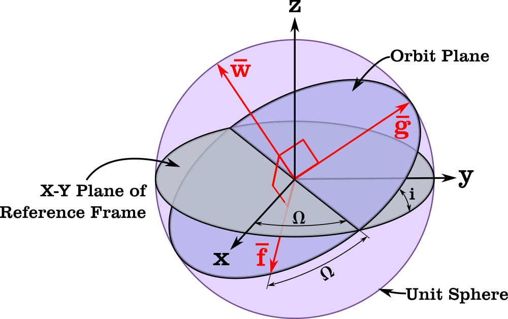
The Orbital Coordinate Frame used for Equinoctial Elements (see Reference [5])
Last time, I mentioned an alternative orbital element set different from the classical elements.
Modified equinoctial elements \((p,f,g,h,k,L)\) are another alternative that are applicable to all orbits and have nonsingular equations of motion (except for a singularity at \(i = \pi\)). They are defined as [1]:
- \(p = a (1 - e^2)\)
- \(f = e \cos (\omega + \Omega)\)
- \(g = e \sin (\omega + \Omega)\)
- \(h = \tan (i/2) \cos \Omega\)
- \(k = \tan (i/2) \sin \Omega\)
- \(L = \Omega + \omega + \nu\)
Where \(a\) is the semimajor axis, \(p\) is the semi-latus rectum, \(i\) is the inclination, \(e\) is the eccentricity, \(\omega\) is the argument of periapsis, \(\Omega\) is the right ascension of the ascending node, \(L\) is the true longitude, and \(\nu\) is the true anomaly. \((f,g)\) are the x and y components of the eccentricity vector in the orbital frame, and \((h,k)\) are the x and y components of the node vector in the orbital frame.
The conversion from Cartesian state (position and velocity) to modified equinoctial elements is given in this Fortran subroutine:
subroutine cartesian_to_equinoctial(mu,rv,evec)

use iso_fortran_env, only: wp => real64

implicit none

real(wp),intent(in)               :: mu    !! central body gravitational parameter (km^3/s^2)
real(wp),dimension(6),intent(in)  :: rv    !! Cartesian state vector
real(wp),dimension(6),intent(out) :: evec  !! Modified equinoctial element vector: [p,f,g,h,k,L]

real(wp),dimension(3) :: r,v,hvec,hhat,ecc,fhat,ghat,rhat,vhat
real(wp) :: hmag,rmag,p,f,g,h,k,L,kk,hh,s2,tkh,rdv

r = rv(1:3)
v = rv(4:6)

rdv      = dot_product(r,v)
rhat     = unit(r)
rmag     = norm2(r)
hvec     = cross(r,v)
hmag     = norm2(hvec)
hhat     = unit(hvec)
vhat     = (rmag*v - rdv*rhat)/hmag
p        = hmag*hmag / mu
k        = hhat(1)/(1.0_wp + hhat(3))
h        = -hhat(2)/(1.0_wp + hhat(3))
kk       = k*k
hh       = h*h
s2       = 1.0_wp+hh+kk
tkh      = 2.0_wp*k*h
ecc      = cross(v,hvec)/mu - rhat
fhat(1)  = 1.0_wp-kk+hh
fhat(2)  = tkh
fhat(3)  = -2.0_wp*k
ghat(1)  = tkh
ghat(2)  = 1.0_wp+kk-hh
ghat(3)  = 2.0_wp*h
fhat     = fhat/s2
ghat     = ghat/s2
f        = dot_product(ecc,fhat)
g        = dot_product(ecc,ghat)
L        = atan2(rhat(2)-vhat(1),rhat(1)+vhat(2))

evec = [p,f,g,h,k,L]

end subroutine cartesian_to_equinoctial
Where cross is a cross product function and unit is a unit vector function (\(\mathbf{u} = \mathbf{v} / |\mathbf{v}|\)).
The inverse routine (modified equinoctial to Cartesian) is:
subroutine equinoctial_to_cartesian(mu,evec,rv)

use iso_fortran_env, only: wp => real64

implicit none

real(wp),intent(in)               :: mu   !! central body gravitational parameter (km^3/s^2)
real(wp),dimension(6),intent(in)  :: evec !! Modified equinoctial element vector : [p,f,g,h,k,L]
real(wp),dimension(6),intent(out) :: rv   !! Cartesian state vector

real(wp) :: p,f,g,h,k,L,s2,r,w,cL,sL,smp,hh,kk,tkh
real(wp) :: x,y,xdot,ydot
real(wp),dimension(3) :: fhat,ghat

p = evec(1)
f = evec(2)
g = evec(3)
h = evec(4)
k = evec(5)
L = evec(6)

kk      = k*k
hh      = h*h
tkh     = 2.0_wp*k*h
s2      = 1.0_wp + hh + kk
cL      = cos(L)
sL      = sin(L)
w       = 1.0_wp + f*cL + g*sL
r       = p/w
smp     = sqrt(mu/p)
fhat(1) = 1.0_wp-kk+hh
fhat(2) = tkh
fhat(3) = -2.0_wp*k
ghat(1) = tkh
ghat(2) = 1.0_wp+kk-hh
ghat(3) = 2.0_wp*h
fhat    = fhat/s2
ghat    = ghat/s2
x       = r*cL
y       = r*sL
xdot    = -smp * (g + sL)
ydot    =  smp * (f + cL)

rv(1:3) = x*fhat + y*ghat
rv(4:6) = xdot*fhat + ydot*ghat

end subroutine equinoctial_to_cartesian
The equations of motion are:
subroutine modified_equinoctial_derivs(mu,evec,scn,evecd)

use iso_fortran_env, only: wp => real64

implicit none

real(wp),intent(in)               :: mu    !! central body gravitational parameter (km^3/s^2)
real(wp),dimension(6),intent(in)  :: evec  !! modified equinoctial element vector : [p,f,g,h,k,L]
real(wp),dimension(3),intent(in)  :: scn   !! Perturbation (in the RSW frame) (km/sec^2)
real(wp),dimension(6),intent(out) :: evecd !! derivative of `evec`

real(wp) :: p,f,g,h,k,L,c,s,n,sqrtpm,sl,cl,s2no2w,s2,w

p      = evec(1)
f      = evec(2)
g      = evec(3)
h      = evec(4)
k      = evec(5)
L      = evec(6)
s      = scn(1)
c      = scn(2)
n      = scn(3)
sqrtpm = sqrt(p/mu)
sl     = sin(L)
cl     = cos(L)
s2     = 1.0_wp + h*h + k*k
w      = 1.0_wp + f*cl + g*sl
s2no2w = s2*n / (2.0_wp*w)

evecd(1) = (2.0_wp*p*c/w) * sqrtpm
evecd(2) = sqrtpm * ( s*sl + ((w+1.0_wp)*cl+f)*c/w - g*n*(h*sl-k*cl)/w )
evecd(3) = sqrtpm * (-s*cl + ((w+1.0_wp)*sl+g)*c/w + f*n*(h*sl-k*cl)/w )
evecd(4) = sqrtpm * s2no2w * cl
evecd(5) = sqrtpm * s2no2w * sl
evecd(6) = sqrt(mu*p)*(w/p)**2 + sqrtpm * ((h*sl-k*cl)*n)/w

end subroutine modified_equinoctial_derivs
The 3-element scn vector contains the components of the perturbing acceleration (e.g. from a thrusting engine, other celestial bodies, etc.) in the directions perpendicular to the radius vector, in the "along track" direction, and the direction of the angular momentum vector.
Integration using modified equinoctial elements will generally be more efficient than a Cowell type integration of the Cartesian state elements. You only have to worry about the one singularity (note that there is also an alternate retrograde formulation where the singularity is moved to \(i = 0\)).
See also
References
- M. J. H. Walker, B. Ireland, Joyce Owens, "A Set of Modified Equinoctial Orbit Elements" Celestial Mechanics, Volume 36, Issue 4, p 409-419. (1985)
- Walker, M. J. H, "Erratum - a Set of Modified Equinoctial Orbit Elements" Celestial Mechanics, Volume 38, Issue 4, p 391-392. (1986)
- Broucke, R. A. & Cefola, P. J., "On the Equinoctial Orbit Elements" Celestial Mechanics, Volume 5, Issue 3, p 303-310. (1972)
- D. A. Danielson, C. P. Sagovac, B. Neta, L. W. Early, "Semianalytic Satellite Theory", Naval Postgraduate School Department of Mathematics, 1995
- P. J. Cefola, "Equinoctial orbit elements - Application to artificial satellite orbits", Astrodynamics Conference, 11-12 September 1972.
Oct 25, 2021
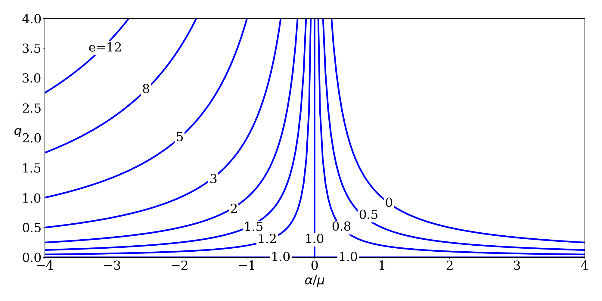
Variation of \(q\) with \(\alpha/\mu ~(=1/a)\) for selected values of \(e\). (see Reference [1])
There are various different 6-element sets that can be used to represent the state (position and velocity) of a spacecraft. The classical Keplerian element set (\(a\), \(e\), \(i\), \(\Omega\), \(\omega\), \(\nu\)) is perhaps the most common, but not the only one. The Gooding universal element set [1] is:
- \(\alpha\) : twice the negative energy per unit mass (\(2 \mu / r - v^2\) or \(\mu/a\))
- \(q\) : periapsis radius magnitude (a.k.a. \(r_p\))
- \(i\) : inclination
- \(\Omega\) : right ascension of the ascending node
- \(\omega\) : argument of periapsis
- \(\tau\) : time since last periapsis passage
The nice thing about this set is that it is always defined, even for parabolas and rectilinear orbits (which other orbital element sets tend to ignore). A table from [1] shows the relationship between \(\alpha\) and \(q\) for the different types of conics:
|
\(\alpha > 0\) |
\(\alpha = 0\) |
\(\alpha < 0\) |
| \(q > 0\) |
general ellipse |
general parabola |
general hyperbola |
| \(q = 0\) |
rectilinear ellipse |
rectilinear parabola |
rectilinear hyperbola |
One advantage of this formulation is for trajectory optimization purposes, since if \(\alpha\) is an optimization variable, the orbit can transition from an ellipse to a hyperbola while iterating without encountering any singularities (which is not true if semimajor axis and eccentricity are being used, since \(a \rightarrow \infty\) for a parabola and then becomes negative for a hyperbola).
Gooding's original paper from 1988 includes Fortran 77 code for the transformations to and from position and velocity, coded with great care to avoid loss of accuracy due to numerical issues. Two other papers [2-3] also include some components of the algorithm. Modernized versions of these routines can be found in the Fortran Astrodynamics Toolkit. For example, a modernized version of ekepl1 (from [2]) for solving Kepler's equation:
pure function ekepl1(em, e)
  !!  Solve kepler's equation, `em = ekepl - e*sin(ekepl)`,
  !!  with legendre-based starter and halley iterator

  implicit none

  real(wp) :: ekepl1
  real(wp),intent(in) :: em
  real(wp),intent(in) :: e

  real(wp) :: c,s,psi,xi,eta,fd,fdd,f

  real(wp),parameter :: testsq = 1.0e-8_wp

  c = e*cos(em)
  s = e*sin(em)
  psi = s/sqrt(1.0_wp - c - c + e*e)

  do
    xi = cos(psi)
    eta = sin(psi)
    fd = (1.0_wp - c*xi) + s*eta
    fdd = c*eta + s*xi
    f = psi - fdd
    psi = psi - f*fd/(fd*fd - 0.5_wp*f*fdd)
    if (f*f < testsq) exit
   end do

   ekepl1 = em + psi

end function ekepl1
The Gooding universal element set can be found in NASA's Copernicus tool, and is being used in the design and optimization of the Artemis I trajectory.
See also
References
- R. H. Gooding, "On universal elements, and conversion procedures to and from position and velocity" Celestial Mechanics 44 (1988), 283-298.
- A. W. Odell, R. H. Gooding, "Procedures for solving Kepler's equation" Celestial Mechanics 38 (1986), 307-334.
- R. H. Gooding, A. W. Odell. "The hyperbolic Kepler equation (and the elliptic equation revisited)" Celestial Mechanics 44 (1988), 267-282.
- J, Williams, J. S. Senent, and D. E. Lee, "Recent improvements to the copernicus trajectory design and optimization system", Advances in the Astronautical Sciences 143, January 2012 (AAS 12-236)
- G. Hintz, "Survey of Orbit Element Sets", Journal of Guidance Control and Dynamics, 31(3):785-790, May 2008
Oct 24, 2021

One of my major pet peeves about Fortran is that it contains virtually no high-level access to the file system. The file system is one of those things that the Fortran standard pretends doesn't exist. It's one of those idiosyncratic things about the Fortran standard, like how it uses the word "processor" instead of "compiler", and doesn't acknowledge the existence of source code files so it doesn't bother to recommend a file extension for Fortran (gotta preserve that backward compatibility just in case punch cards come back).
There are various hacky workarounds to do various things that poor Fortran programmers have had to use for decades. Basically, all you have is OPEN, CLOSE, READ, WRITE, and INQUIRE. Here are a few examples:
Deleting a file
Here's a standard Fortran routine that can be used to delete a file:
function delete_file(name) result(istat)

  implicit none

  character(len=*),intent(in) :: name
  integer :: istat

  integer :: iunit

  open(newunit=iunit,status='OLD',iostat=istat)
  if (istat==0) close(iunit,status='DELETE',iostat=istat)

end function delete_file
As you can see, it's just a little trick, using a feature of CLOSE to delete a file after closing it (but first, we had to open it). Of course, note that the error codes are non-standard (the Fortran standard also doesn't consider this information important and lets the different compilers do whatever they want -- so of course, they all do something different). And of course, there is no exception handling in Fortran either (a post for another time).
Creating a directory
There is absolutely no standard ability in Fortran to create or delete a directory. Again, Fortran basically pretends that directories don't exist. Note that the Intel Fortran Compiler provides a super useful non-standard extension of the INQUIRE statement to allow it to be used to get information about directories. It's a pretty ridiculous state of affairs (Fortran added a bazillion IEEE routines in Fortran 2018 for some reason that nobody needed, but it still doesn't have something like this that everybody has needed for decades). Intel's IFPORT portability module provides many useful (non-standard) routines for accessing the file system (for example DELFILESQQ for deleting files and DELDIRQQ for deleting a directory). I use these all the time and the fact that they are non-standard and not present in other compilers is a major source of annoyance.
For some file or directory operations, you can always resort to using system calls, and thus have to provide different methods for different platforms (of course Fortran provides no standard way to get any information about the platform, so you have to resort to non-standard, possibly compiler-specific, preprocessor directives to do that). For example, to create a directory you could use:
subroutine make_directory(name)

  implicit none

  character(len=*),intent(in) :: name

  call execute_command_line ('mkdir '//name)

end subroutine make_directory
That one was easy because "mkdir" works on macOS, Window, and Linux. See previous post about getting command line calls into strings, which can also be useful for some things like this.
Getting a list of files
How about getting a list of all the files that match a specific pattern? Again, this can be done if you are using the Intel compiler using the IFPORT module GETFILEINFOQQ routine:
function get_filenames(pattern, maxlen) result(list)

  use ifport

  implicit none

  character(len=*),intent(in) :: pattern
  integer,intent(in) :: maxlen
  character(len=maxlen),dimension(:),allocatable :: list

  integer(kind=int_ptr_kind()) :: handle
  type(file$infoi8) :: info
  integer :: length

  allocate(list(0))
  handle = file$first
  do
    length = GETFILEINFOQQ(trim(pattern), info, handle)
    if ((handle==file$last) .or. (handle==file$error)) exit
    list = [list, info%name]
  end do

end function get_filenames
The file$infoi8 type is some super-weird non-standard Intel thing. Note that this example only returns the file names, not the full paths. To get the full path is left as an exercise to the reader. Also note that Fortran doesn't provide a good string class, so we just set a maximum string length as an argument to this function (but note that Intel is only returning a 255-character string anyway).
Final thoughts
There are various libraries out there that can do some of this. For example, M_system (a Fortran module interface for calling POSIX C system routines). Hopefully, a comprehensive set of filsystem routines will eventually make it into the Fortran Standard Library.
See also