Sorting with Magic Numbers
Updated July 7, 2014
Poorly commented sourcecode is one of my biggest pet peeves. Not only should the comments explain what the routine does, but where the algorithm came from and what its limitations are. Consider ISORT, a non-recursive quicksort routine from SLATEC, written in 1976. In it, we encounter the following code:
R = 0.375E0
...
IF (R .LE. 0.5898437E0) THEN
    R = R+3.90625E-2
ELSE
    R = R-0.21875E0
ENDIF
What are these magic numbers? An internet search for "0.5898437" yields dozens of hits, many of them different versions of this algorithm translated into various other programming languages (including C, C++, and free-format Fortran). Note: the algorithm here is the same one, but also prefaces this code with the following helpful comment:
! And now...Just a little black magic...
Frequently, old code originally written in single precision can be improved on modern computers by updating to full-precision constants (replacing 3.14159 with a parameter computed at compile time as acos(-1.0_wp) is a classic example). Is this the case here? Sometimes WolframAlpha is useful in these circumstances. It tells me that a possible closed form of 0.5898437 is: \(\frac{57}{100\pi}+\frac{13\pi}{100} \approx 0.58984368009\). Hmmmmm... The reference given in the header is no help [1], it doesn't contain this bit of code at all.
It turns out, what this code is doing is generating a pseudorandom number to use as the pivot element in the quicksort algorithm. The code produces the following repeating sequence of values for R:
0.375
0.4140625
0.453125
0.4921875
0.53125
0.5703125
0.609375
0.390625
0.4296875
0.46875
0.5078125
0.546875
0.5859375
0.625
0.40625
0.4453125
0.484375
0.5234375
0.5625
0.6015625
0.3828125
0.421875
0.4609375
0.5
0.5390625
0.578125
0.6171875
0.3984375
0.4375
0.4765625
0.515625
0.5546875
0.59375
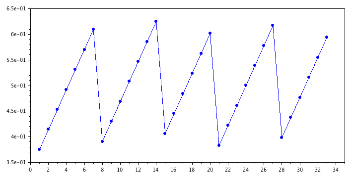
This places the pivot point near the middle of the set. The source of this scheme is from Reference [2], and is also mentioned in Reference [3]. According to [2]:
These four decimal constants, which are respectively 48/128, 75.5/128, 28/128, and 5/128, are rather arbitrary.
The other magic numbers in this routine are the dimensions of these variables:
INTEGER IL(21), IU(21)
These are workspace arrays used by the subroutine, since it does not employ recursion. But, since they have a fixed size, there is a limit to the size of the input array this routine can sort. What is that limit? You would not know from the documentation in this code. You have to go back to the original reference [1] (where, in fact, these arrays only had 16 elements). There, it explains that the arrays IL(K) and IU(K) permit sorting up to \(2^{k+1}-1\) elements (131,071 elements for the k=16 case). With k=21, that means the ISORT routine will work for up to 4,194,303 elements. So, keep that in mind if you are using this routine.
There are many other implementations of the quicksort algorithm (which was declared one of the top 10 algorithms of the 20th century). In the LAPACK quicksort routine DLASRT, k=32 and the "median of three" method is used to select the pivot. The quicksort method in R is the same algorithm as ISORT, except that k=40 (this code also has the advantage of being properly documented, unlike the other two).
References
- R. C. Singleton, "Algorithm 347: An Efficient Algorithm for Sorting With Minimal Storage", Communications of the ACM, Vol. 12, No. 3 (1969).
- R. Peto, "Remark on Algorithm 347", Communications of the ACM, Vol. 13 No. 10 (1970).
- R. Loeser, "Survey on Algorithms 347, 426, and Quicksort", ACM Transactions on Mathematical Software (TOMS), Vol. 2 No. 3 (1976).