May 30, 2016
Sorting is one of the fundamental problems in computer science, so of course Fortran does not include any intrinsic sorting routine (we've got Bessel functions, though!) String sorting is a special case of this problem which includes various choices to consider, for example:
- Natural or ASCII sorting
- Case sensitive (e.g., 'A'<'a') or case insensitive (e.g., 'A'=='a')
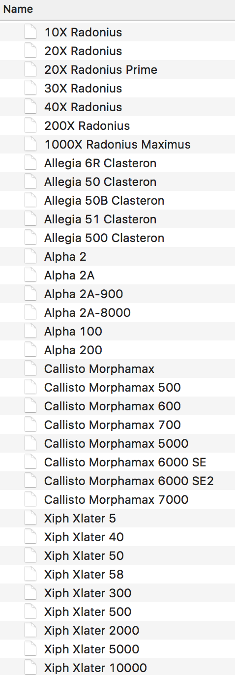
"Natural" sorting (also called "alphanumeric sorting" means to take into account numeric values in the string, rather than just comparing the ASCII value of each of the characters. This can produce an order that looks more natural to a human for strings that contain numbers. For example, in a "natural" sort, the string "case2.txt" will come before "case100.txt", since the number 2 comes before the number 100. For example, natural sorting is the method used to sort file names in the MacOS X Finder (see image at right). While, interestingly, an ls -l from a Terminal merely does a basic ASCII sort.
For string sorting routines written in modern Fortran, check out my GitHub project stringsort. This library contains routines for both natural and ASCII string sorting. Natural sorting is achieved by breaking up each string into chunks. A chunk consists of a non-numeric character or a contiguous block of integer characters. A case insensitive search is done by simply converting each character to lowercase before comparing them. I make no claim that the routines are particularly optimized. One limitation is that contiguous integer characters are stored as an integer(INT32) value, which has a maximum value of 2147483647. Although note that it is easy to change the code to use integer(INT64) variables to increase this range up to 9223372036854775807 if necessary. Eliminating integer size restrictions entirely is left as an exercise for the reader.
Consider the following test case:
character(len=*),dimension(6) :: &
str = [ 'z1.txt ', &
        'z102.txt', &
        'Z101.txt', &
        'z100.txt', &
        'z10.txt ', &
        'Z11.txt ' ]
This list can be sorted (at least) four different ways:
Case Insensitive
ASCII
z1.txt
z10.txt
z100.txt
Z101.txt
z102.txt
Z11.txt
natural
z1.txt
z10.txt
Z11.txt
z100.txt
Z101.txt
z102.txt
Case Sensitive
ASCII
Z101.txt
Z11.txt
z1.txt
z10.txt
z100.txt
z102.txt
natural
Z11.txt
Z101.txt
z1.txt
z10.txt
z100.txt
z102.txt
Each of these can be done using stringsort with the following subroutine calls:
call lexical_sort_recursive(str,case_sensitive=.false.)
call lexical_sort_natural_recursive(str,case_sensitive=.false.)

call lexical_sort_recursive(str,case_sensitive=.true.)
call lexical_sort_natural_recursive(str,case_sensitive=.true.)
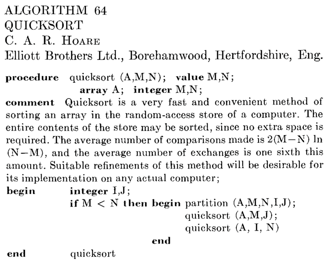
*Original Quicksort algorithm by Tony Hoare, 1961 (Communications of the ACM)*
The routines use the quicksort algorithm, which was originally created for sorting strings (specifically words in Russian sentences so they could be looked up in a Russian-English dictionary). The algorithm is easily implemented in modern Fortran using recursion (non-recursive versions were also available before recursion was added to the language in Fortran 90). Quicksort was named one of the top 10 algorithms of the 20th century by the ACM (Fortran was also on the list).
See also
May 17, 2015
Topological sorting can be used to determine the order in which a collection of interdependent tasks must be performed. For example, when building a complex modern Fortran application, there can be many modules with complex interdependencies (via use association). A Fortran building system (like FoBiS, Foray, or SCons) will perform a topological sort to determine the correct compilation order. In graph theory, the collection of tasks are vertices of a directed graph. If there are no circular dependencies, then it is a directed acyclic graph (DAG).
An example modern Fortran implementation of a topological sorting algorithm is given here. The only public class is dag, which is used to define the graph and perform the sort. The toposort method performs a "depth-first" traversal of the graph using the recursive subroutine dfs. Each vertex is only visited once, and so the algorithm runs in linear time. The routine also triggers an error message for circular dependencies.
module toposort_module
!! Topological sorting, using a recursive
!! depth-first method. The vertices are
!! integer values from (1, 2, ..., nvertices)

implicit none

private

type :: vertex
    !! a vertex of a directed acyclic graph (DAG)
    integer,dimension(:),allocatable :: edges
    integer :: ivertex = 0 !vertex number
    logical :: checking = .false.
    logical :: marked = .false.
    contains
    procedure :: set_edges
end type vertex

type,public :: dag
    !! a directed acyclic graph (DAG)
    type(vertex),dimension(:),allocatable :: vertices
    contains
    procedure :: set_vertices => dag_set_vertices
    procedure :: set_edges => dag_set_edges
    procedure :: toposort => dag_toposort
end type dag

contains

subroutine set_edges(me,edges)
    !! specify the edge indices for this vertex
    implicit none
    class(vertex),intent(inout) :: me
    integer,dimension(:),intent(in) :: edges
    allocate(me%edges(size(edges)))
    me%edges = edges
end subroutine set_edges

subroutine dag_set_vertices(me,nvertices)
    !! set the number of vertices in the dag
    implicit none
    class(dag),intent(inout) :: me
    integer,intent(in) :: nvertices !! number of vertices
    integer :: i
    allocate(me%vertices(nvertices))
    me%vertices%ivertex = [(i,i=1,nvertices)]
end subroutine dag_set_vertices

subroutine dag_set_edges(me,ivertex,edges)
    !! set the edges for a vertex in a dag
    implicit none
    class(dag),intent(inout) :: me
    integer,intent(in) :: ivertex !! vertex number
    integer,dimension(:),intent(in) :: edges
    call me%vertices(ivertex)%set_edges(edges)
end subroutine dag_set_edges

subroutine dag_toposort(me,order)
    !! main toposort routine

    implicit none

    class(dag),intent(inout) :: me
    integer,dimension(:),allocatable,intent(out) :: order

    integer :: i,n,iorder

    n = size(me%vertices)
    allocate(order(n))
    iorder = 0 ! index in order array
    do i=1,n
        if (.not. me%vertices(i)%marked) &
            call dfs(me%vertices(i))
    end do

contains

    recursive subroutine dfs(v)
        !! depth-first graph traversal

        type(vertex),intent(inout) :: v

        integer :: j

        if (v%checking) then
            error stop 'Error: circular dependency.'
        else
            if (.not. v%marked) then
                v%checking = .true.
                if (allocated(v%edges)) then
                    do j=1,size(v%edges)
                        call dfs(me%vertices(v%edges(j)))
                    end do
                end if
                v%checking = .false.
                v%marked = .true.
                iorder = iorder + 1
                order(iorder) = v%ivertex
            end if
        end if

    end subroutine dfs

end subroutine dag_toposort

end module toposort_module
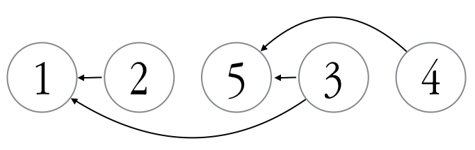
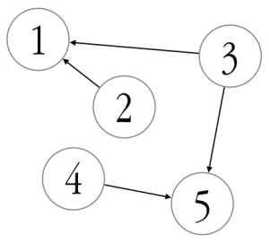
An example use of this module is given below. Here, we define a graph with five vertices: task 2 depends on 1, task 3 depends on both 1 and 5, and task 4 depends on 5.
program main

    use toposort_module
    implicit none

    type(dag) :: d
    integer,dimension(:),allocatable :: order

    call d%set_vertices(5)
    call d%set_edges(2,[1])   ! 2 depends on 1
    call d%set_edges(3,[5,1]) ! 3 depends on 5 and 1
    call d%set_edges(4,[5])   ! 4 depends on 5
    call d%toposort(order)

    write(*,*) order

end program main
The result is:

Which is the evaluation order. As far as I can find, the above code is the only modern Fortran topological sorting implementation available on the internet. There is a FORTRAN 77 subroutine here, and a Fortran 90-ish one here (however, neither of them check for circular dependencies).
See also
- Topological Sorting [Everything Under The Sun], June 26, 2013.
- Topological sorting [Wikipedia]
- tsort -- UNIX command for performing topological sorting. [Note that this gives the result in the reverse order from the code listed above.]
Jul 05, 2014
Updated July 7, 2014
Poorly commented sourcecode is one of my biggest pet peeves. Not only should the comments explain what the routine does, but where the algorithm came from and what its limitations are. Consider ISORT, a non-recursive quicksort routine from SLATEC, written in 1976. In it, we encounter the following code:
R = 0.375E0
...
IF (R .LE. 0.5898437E0) THEN
    R = R+3.90625E-2
ELSE
    R = R-0.21875E0
ENDIF
What are these magic numbers? An internet search for "0.5898437" yields dozens of hits, many of them different versions of this algorithm translated into various other programming languages (including C, C++, and free-format Fortran). Note: the algorithm here is the same one, but also prefaces this code with the following helpful comment:
! And now...Just a little black magic...
Frequently, old code originally written in single precision can be improved on modern computers by updating to full-precision constants (replacing 3.14159 with a parameter computed at compile time as acos(-1.0_wp) is a classic example). Is this the case here? Sometimes WolframAlpha is useful in these circumstances. It tells me that a possible closed form of 0.5898437 is: \(\frac{57}{100\pi}+\frac{13\pi}{100} \approx 0.58984368009\). Hmmmmm... The reference given in the header is no help [1], it doesn't contain this bit of code at all.
It turns out, what this code is doing is generating a pseudorandom number to use as the pivot element in the quicksort algorithm. The code produces the following repeating sequence of values for R:
0.375
0.4140625
0.453125
0.4921875
0.53125
0.5703125
0.609375
0.390625
0.4296875
0.46875
0.5078125
0.546875
0.5859375
0.625
0.40625
0.4453125
0.484375
0.5234375
0.5625
0.6015625
0.3828125
0.421875
0.4609375
0.5
0.5390625
0.578125
0.6171875
0.3984375
0.4375
0.4765625
0.515625
0.5546875
0.59375
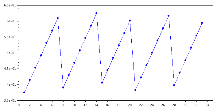
This places the pivot point near the middle of the set. The source of this scheme is from Reference [2], and is also mentioned in Reference [3]. According to [2]:
These four decimal constants, which are respectively 48/128, 75.5/128, 28/128, and 5/128, are rather arbitrary.
The other magic numbers in this routine are the dimensions of these variables:
These are workspace arrays used by the subroutine, since it does not employ recursion. But, since they have a fixed size, there is a limit to the size of the input array this routine can sort. What is that limit? You would not know from the documentation in this code. You have to go back to the original reference [1] (where, in fact, these arrays only had 16 elements). There, it explains that the arrays IL(K) and IU(K) permit sorting up to \(2^{k+1}-1\) elements (131,071 elements for the k=16 case). With k=21, that means the ISORT routine will work for up to 4,194,303 elements. So, keep that in mind if you are using this routine.
There are many other implementations of the quicksort algorithm (which was declared one of the top 10 algorithms of the 20th century). In the LAPACK quicksort routine DLASRT, k=32 and the "median of three" method is used to select the pivot. The quicksort method in R is the same algorithm as ISORT, except that k=40 (this code also has the advantage of being properly documented, unlike the other two).
References
- R. C. Singleton, "Algorithm 347: An Efficient Algorithm for Sorting With Minimal Storage", Communications of the ACM, Vol. 12, No. 3 (1969).
- R. Peto, "Remark on Algorithm 347", Communications of the ACM, Vol. 13 No. 10 (1970).
- R. Loeser, "Survey on Algorithms 347, 426, and Quicksort", ACM Transactions on Mathematical Software (TOMS), Vol. 2 No. 3 (1976).