Jun 14, 2026
The FMIN function at Netlib is based on Richard Brent's classic localmin algorithm from [1].
The method uses a combination of golden section search and successive parabolic interpolation to compute the minimum of a 1D function without the necessity of evaluating any derivatives. There are Fortran 66 and ALGOL 60 versions of the method in the reference. I also have a modernized version here.
Let's show an example of how to use it for a simple orbital mechanics application.
Problem setup
Let's solve a trivial problem in orbital mechanics: computing the time of closest approach to a planet for a conic orbit. This is known as periapsis (or, for the Earth, perigee). We don't really need to use a minimizer to compute this, but it's a problem with a known solution that we can test the minimizer on.
We need various algorithms to do this:
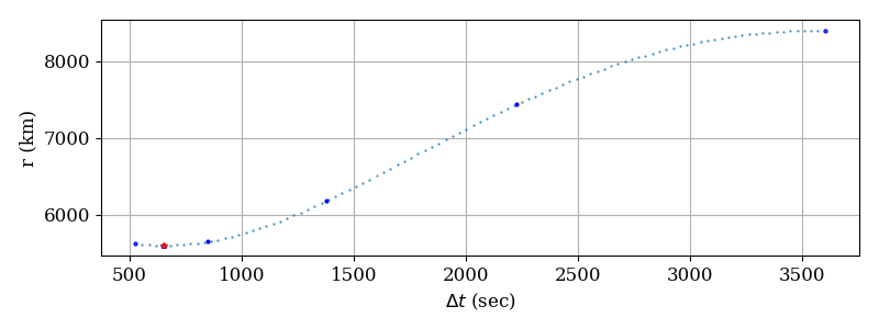
Given an initial elliptical orbit state, the Gooding routine pv3els will compute the time since last periapsis passage, so we have the "true" value to compare the results against. The function we pass to fmin to minimize will simply propagate the state (the independent variable is \(\Delta t\)) and return the radius magnitude (\(r\)). The point where the radius magnitude is minimized is the periapsis point we are looking for. The orbital period is used to set the upper time bound for the minimizer (we know there is only one periapsis passage per orbital period).
Example code
In our Fortran Package Manager manifest file, we define the two external dependencies we need:
[dependencies]
fmin = { git="https://github.com/jacobwilliams/fmin.git" }
fortran-astrodynamics-toolkit = { git="https://github.com/jacobwilliams/fortran-astrodynamics-toolkit.git" }
And the main program looks like this:
program main
  use fmin_module, wp => fmin_rk
  use fortran_astrodynamics_toolkit

  implicit none

  real(wp) :: p !! semiparameter [km]
  real(wp) :: period !! orbital period [sec]
  real(wp) :: dt !! time from initial state to periapsis [sec]
  real(wp),dimension(3) :: r, v !! position and velocity vectors [km] and [km/s]
  real(wp),dimension(6) :: rv0 !! initial state vector [km, km/s]
  real(wp),dimension(6) :: e0 !! Gooding orbital elements of the initial state
  integer :: n_evals = 0 !! number of function evaluations

  ! initial conditions (orbital elements):
  real(wp),parameter :: mu   = 398600.4418_wp  !! Earth grav. parameter [km^3/s^2]
  real(wp),parameter :: a    = 7000.0_wp       !! semi-major axis [km]
  real(wp),parameter :: ecc  = 0.2_wp          !! eccentricity
  real(wp),parameter :: inc  = 30.0_wp         !! inclination [deg]
  real(wp),parameter :: raan = 40.0_wp         !! right ascension of ascending node [deg]
  real(wp),parameter :: aop  = 60.0_wp         !! argument of perigee [deg]
  real(wp),parameter :: tru  = -45.0_wp        !! true anomaly [deg]
  real(wp),parameter :: tol  = 1.0e-6_wp       !! tolerance for fmin

  ! get the initial state vector and time from periapsis for the initial state:
  p = a * (1.0_wp - ecc**2)
  period = orbit_period(mu,a)
  call orbital_elements_to_rv(mu, p, ecc, inc, raan, aop, tru, r, v)
  rv0 = [r, v]
  call pv3els (mu, rv0, e0) ! e0(6) is the time from periapsis of the initial state

  ! call the minimizer:
  dt = fmin(func,0.0_wp,period,tol)

  ! print results
  write(*,'(A,F12.6,A)') 'DT to periapsis from fmin        = ', dt, ' sec'
  write(*,'(A,F12.6,A)') 'True initial time from periapsis = ', e0(6), ' sec'
  write(*,'(A,E12.3,A)') 'Error                            = ', dt + e0(6), ' sec'
  write(*,'(A,I0,A)')    'number of function evals         = ', n_evals, ' '

  contains

  function func(x) result(f)
    !! the function is to propagate from the initial state
    !! by the dt and compute the radius value
    real(wp),intent(in) :: x  !! indep. variable (dt)
    real(wp)            :: f  !! function value `f(x)` - radius magnitude
    real(wp),dimension(6) :: rvf
    call propagate(mu, rv0, x, rvf)
    f = norm2(rvf(1:3))
    n_evals = n_evals + 1
  end function func

end program main
Easy peasy!
Results
The result of running this program is:
DT to periapsis from fmin        =   652.983248 sec
True initial time from periapsis =  -652.983240 sec
Error                            =    0.875E-05 sec
number of function evals         = 12
So, it works! Using 12 function evaluations (i.e., kepler propagations of the orbit), the method has located the periapsis time to within about 8 \(\mu s\).
This sort of approach can also be used for less-trivial problems where we don't have a good analytical solution, and/or derivatives are unavailable or hard to obtain.
References
- R. Brent, "Algorithms for Minimization Without Derivatives", Prentice-Hall, 1973.
Jun 13, 2026

Reference [1] describes a numerical method for computing the derivative of a 1D function, using Neville's algorithm to extrapolate from a sequence of simple polynomial approximations based on interpolating points within specific bounds of a given point.
The original code in the published paper in 1980 was written in ALGOL 60. It seems as if a Fortran 77 translation was produced by David Kahaner at NIST circa 1989. I found the file on this NIST server where it has been sitting quietly since 1992 (originally this was an ftp server when I first found it). It's an interesting algorithm, and I included a modernized version in my NumDiff numerical differentiation library.
I also note that a version of the code is embedded within the Dataplot package.
But, there is a problem!
Here is a line of code in the original faccuracy function:
IF 16*ABS(H1)>ABS(H0) THEN H1:=SIGN(H1)*ABS(H0)/16;
Now, I know nothing about ALGOL 60, except that apparently John Backus (the creator of Fortran) was one of the committee members that developed it. Notice the SIGN function in this code.
This line was translated into Fortran 77 (where the function is renamed as FACCUR) as:
IF(16.*ABS(H1) .GT. ABS(H0)) H1 = SIGN(H1,1.)*ABS(H0)/16.
They are very similar, but note the SIGN function again.
In Fortran, the SIGN function (added in Fortran 77) is a little different since it has two arguments. While more flexible, it is a never-ending source of confusion, and I always have to look up the meaning of the two arguments. The following table summarizes the difference between the two:
| Language |
Syntax |
Description |
Reference |
| ALGOL 60 |
sign(E) |
the sign of the value of E (+1 for E>0, 0 for E=0, -1 for E<0) |
[2] |
| Fortran |
sign(A, B) |
the value of A with the sign of B |
[3] |
So, do you see the bug? SIGN(H1,1.) doesn't return the same thing that SIGN(H1) did in the original code. SIGN(H1,1.) returns the value of H1 with the sign of 1.0, which is always +H1, not the original intent at all! It really should have been translated to SIGN(1.0,H1), to give the +1/-1 of the original code. So, this bug is over 30 years old. Technically, the 0 case is still not handled the same, but that's a degenerate case that would never happen or give meaningful results in this context. But to be totally faithful we would need to use a function like this:
elemental real(wp) function sign_algol(x)
real(wp),intent(in) :: x
sign_algol = merge(0.0_wp, sign(1.0_wp,x), x==0.0_wp)
end function sign_algol
Other Languages
Python doesn't have a built-in sign function, but the numpy one behaves exactly like the ALGOL one. The advantage of the Fortran one is that it does support signed zeros, which the Numpy one does not appear to support (for that you need to use copysign). C++ also has a copysign function that does the same thing.
References
- J. Oliver, "Algorithm 017: An algorithm for numerical differentiation of a function of one real variable", Journal of Computational and Applied Mathematics 6 (2) (1980) 145-160. Fortran 77 code from NIST.
- J. W. Backus, F. L. Bauer, J. Green, C. Katz, J. McCarthy, A. J. Perlis, H. Rutishauser, K. Samelson, B. Vauquois, J. H. Wegstein, A. van Wijngaarden, M. Woodger Editor: P. Naur, "Revised Report on the Algorithmic Language ALGOL 60", Communications of the ACM, Volume 6, Issue 1
Pages 1 - 17, 01 January 1963.
- SIGN — Sign copying function [gcc.gnu.org]
- Numerical Differentiation, degenerateconic.com, Dec 04, 2016
May 30, 2026
Consider the problem of finding all the roots of a polynomial. This involves solving the following equation:
$$a_0 + a_1 x + a_2 x^2 + \cdots + a_n x^n = 0$$
This problem occurs in many different applications, such as computing atmospheric density in a spacecraft orbit simulation.
In general, both the coefficients and roots can be complex numbers. A special case involves only real coefficients. General methods exist for any degree polynomial, and custom methods also exist for polynomials of specific degree. The quadratic formula is the most famous analytical solution for polynomials of degree 2. In general, numerical methods are necessary to solve polynomials of degree 5 and higher.
Newton's method is frequently used, which requires an initial guess and an iterative procedure. Another elegant way to solve for all the roots at once is to find the eigenvalues of the companion matrix.
Fortran library

My polyroots-fortran library includes various methods to solve this problem. Many of the implementations have legacy going back decades (for example, from SLATEC). It's easy to incorporate into other codes using the Fortran Package Manager.
The available methods in the library are:
Example
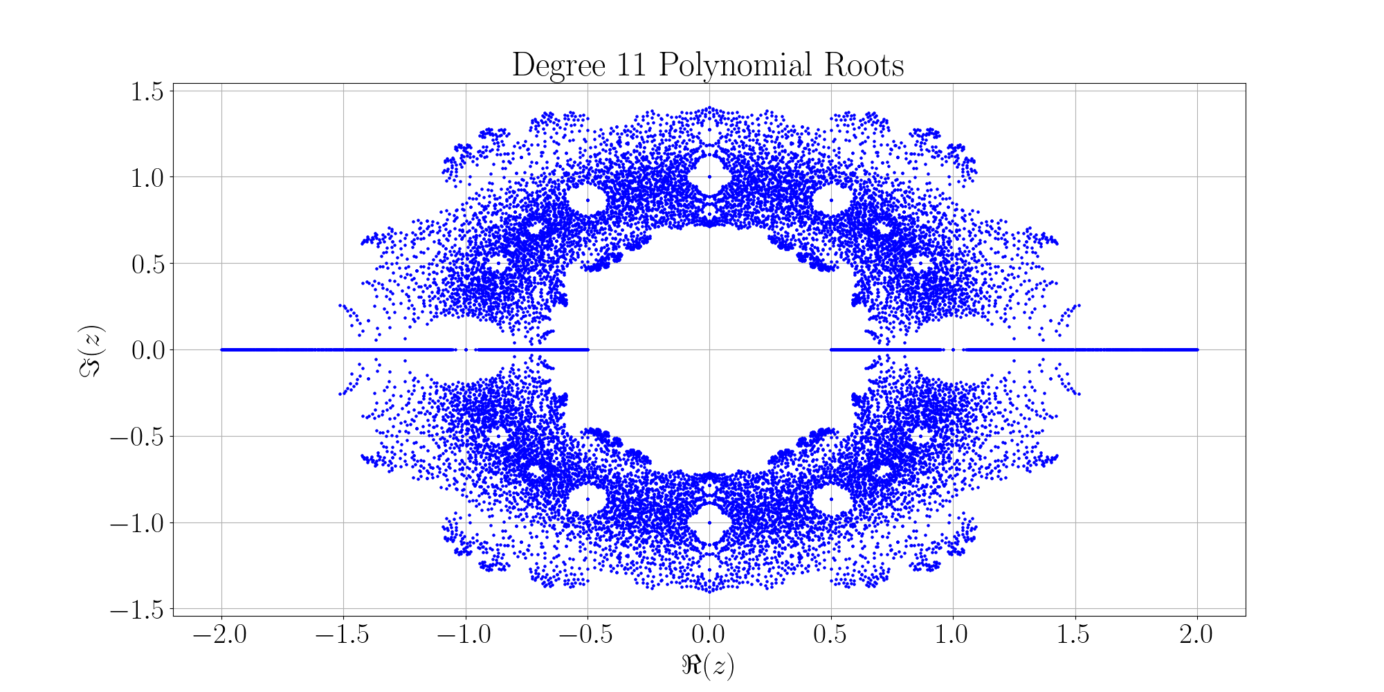
As an example, let's generate a plot of all the roots for all \(11^{th}\) degree polynomials with coefficients either +1 or -1. That is:
| \(a_0\) |
\(a_1\) |
\(a_2\) |
\(a_3\) |
\(a_4\) |
\(a_5\) |
\(a_6\) |
\(a_7\) |
\(a_8\) |
\(a_9\) |
\(a_{10}\) |
\(a_{11}\) |
| -1 |
-1 |
-1 |
-1 |
-1 |
-1 |
-1 |
-1 |
-1 |
-1 |
-1 |
-1 |
| -1 |
-1 |
-1 |
-1 |
-1 |
-1 |
-1 |
-1 |
-1 |
-1 |
-1 |
1 |
| -1 |
-1 |
-1 |
-1 |
-1 |
-1 |
-1 |
-1 |
-1 |
-1 |
1 |
-1 |
| -1 |
-1 |
-1 |
-1 |
-1 |
-1 |
-1 |
-1 |
-1 |
-1 |
1 |
1 |
| -1 |
-1 |
-1 |
-1 |
-1 |
-1 |
-1 |
-1 |
-1 |
1 |
-1 |
-1 |
| -1 |
-1 |
-1 |
-1 |
-1 |
-1 |
-1 |
-1 |
-1 |
1 |
-1 |
1 |
| -1 |
-1 |
-1 |
-1 |
-1 |
-1 |
-1 |
-1 |
-1 |
1 |
1 |
-1 |
| -1 |
-1 |
-1 |
-1 |
-1 |
-1 |
-1 |
-1 |
-1 |
1 |
1 |
1 |
| \(\vdots\) |
\(\vdots\) |
\(\vdots\) |
\(\vdots\) |
\(\vdots\) |
\(\vdots\) |
\(\vdots\) |
\(\vdots\) |
\(\vdots\) |
\(\vdots\) |
\(\vdots\) |
\(\vdots\) |
| 1 |
1 |
1 |
1 |
1 |
1 |
1 |
1 |
1 |
1 |
1 |
1 |
We'll use the polyroots method, which solves for the roots of a real polynomial equation by computing the eigenvalues of the companion matrix (using the LAPACK eigen solver DGEEV).
To get all the coefficient permutations, we will use a recursive algorithm, and pyplot-fortran to generate the plot.
Here is the code:
program main

use polyroots_module, only: polyroots, wp => polyroots_module_rk
use pyplot_module,    only: pyplot

implicit none

integer,parameter :: degree = 11 !! polynomial degree
integer,dimension(2) :: icoeffs = [-1,1] !! set of coefficients
integer,dimension(degree+1) :: a !! coefficients of polynomial
type(pyplot) :: plt  !! for making the plot
integer      :: ierr !! error code from [[polyroots]]
integer      :: j    !! counter

call plt%initialize(grid=.true.,xlabel='$\\Re(z)$',ylabel='$\\Im(z)$',&
                    title='Degree 11 Polynomial Roots',usetex=.true.,&
                    font_size=30, axes_labelsize=30, &
                    xtick_labelsize=30, ytick_labelsize=30, &
                    figsize=[20,10])
call generate(1)
call plt%showfig()

contains

    recursive subroutine generate(i)
    integer, intent(in) :: i
    integer :: ix
    real(wp),dimension(degree) :: zr, zi !! roots
    if (i > degree+1) then
        ! solve for this root and add it to the plot:
        call polyroots(degree,real(a,wp),zr,zi,ierr)
        call plt%add_plot(zr,zi,label='',linestyle='bo',markersize=2)
    else
        do ix = 1,size(icoeffs)
            a(i) = icoeffs(ix)
            call generate(i+1)
        end do
    end if
    end subroutine generate

end program main
The first set of roots, for \(a = [-1,-1,-1,-1,-1,-1,-1,-1,-1,-1,-1,-1]\), are: [\(-1\), \(\pm i\), \(\pm \sqrt3/2 \pm 0.5 i\), \(\pm 0.5 \pm \sqrt3/2\)].
The resultant plot with all the roots is shown here:
References
May 25, 2026
"I am bound Upon a wheel of fire, that mine own tears Do scald like molten lead." - Shakespeare, "King Lear", Act IV, Scene 7
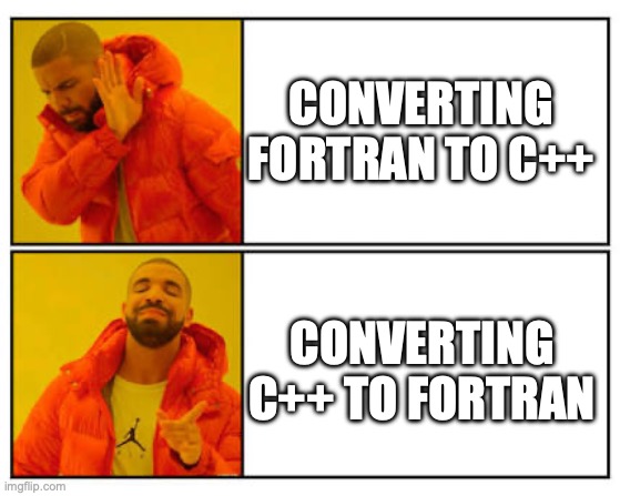
Typically, we see examples of poor saps who think that legacy Fortran codes must be converted to "modern" languages such as C++.
Well, let's try to do the reverse! Let's try converting some "legacy" C++ code to modern Fortran. The example I will show is the Jacchia-Roberts atmosphere model from GMAT (General Mission Analysis Tool). This model is widely used for satellite orbit simulations to model satellite drag. There is no modern Fortran implementation publicly available as far as I can tell, so let's create one.
And just to see what happens, I'll do this with assistance from AI, particularly Claude Sonnet (initially 4.5, but also trying 4.6) in GitHub Copilot. What could go wrong?
All About the Vibes
First, we start with the C++ files we want to convert. These files are at least 20 years old, with heritage going back even further. The main ones are:
- JacchiaRobertsAtmosphere.cpp - the main implementation of the Jacchia-Roberts density model.
- SolarFluxReader.cpp - the algorithm to read in a space weather file. There are a couple different file formats supported here, but I'm only going to worry about the CSSI one.
- A1Mjd.cpp - Some time conversion routines. This will be important later when trying to diagnose some validation issues.
Using AI is a very interesting and also frustrating experience.
It's like working with someone who is a genius, but is also an idiot and sometimes a compulsive liar.
The initial conversion got me 80% of the way there but was subtly wrong in various ways.
I started with a basic prompt ("Convert this C++ file into modern Fortran") and went from there.
There was a lot of back and forth and manual interventions to fix little issues (syntax errors, etc.)
In one instance, I tried to get it to identify the source of a bug, and it "thought" for 15 minutes until I finally just gave up and looked at the code myself and fixed it instantly.
Sometimes, it would get fixated on one approach that wasn't correct, and I'd have to keep telling it to ignore that approach and try something else (e.g., I had to figure out the correct way to do something, and once I gave it more directions, it was fine and could do it).
One thing that was annoying was that it kept trying to generate code from first principles rather than performing a straight up conversion of the C++ code to Fortran. I had to keep reminding it that what I wanted was a faithful translation.
At one point, I switched to Sonnet 4.6 and it also found a couple of code typos that Sonnet 4.5 had generated.
The Result
See jacchia-roberts-fortran for the end result. The library provides a class that can be used to initialize the model with a given space weather file (or constant values can be specified). Then a method is provided for computing the density.
An example use case is:
program example

use jacchia_roberts_module, only: jacchia_roberts_type
use jacchia_roberts_kinds,  only: ip, dp

implicit none

type(jacchia_roberts_type) :: jr
integer(ip) :: status
real(dp) :: density

! example inputs:
real(dp),parameter :: rad_earth = 6356.766_dp ! Earth polar radius (km)
character(len=*),parameter :: sw_file = 'data/SpaceWeather-All-v1.2.txt' ! space weather file to load
real(dp),parameter :: utc_mjd = 59215.5_dp ! MJD: Jan 1, 2021 12:00 UTC
real(dp),parameter :: alt_km = 200.0_dp ! geodetic altitude (km)
real(dp),parameter :: lat = 20.0_dp ! geodetic latitude (deg)
real(dp),dimension(3),parameter :: r = [7000.0_dp, 0.0_dp, 0.0_dp] ! spacecraft position vector (km)
real(dp),dimension(3),parameter :: sun = [1.0_dp, 0.0_dp, 0.0_dp] ! sun direction unit vector

! initialize the model:
call jr%initialize(rad_earth, filename=sw_file, status=status)

! compute the density:
density = jr%density(alt_km, r, sun_vector, lat, utc_mjd)

end program example
The idea is, first you would initialize the class, and then during your simulation, call the model to get the atmospheric density using the current epoch and state of the spacecraft. A flow chart of the process would look a little like this:

The resultant Fortran code is very clean compared to the C++ code. Consider this example (the rho_cor function). The original C++ code:
Real JacchiaRobertsAtmosphere::rho_cor(Real height, Real a1_time, Real geo_lat,
                                       GEOPARMS *geo)
{
   Real geo_cor, semian_cor, slat_cor, f, g, day_58, tausa, alpha;
   Real sin_lat, eta_lat;

   // Compute geomagnetic activity correction
   if (height < 200.0)
   {
      geo_cor = 0.012 * geo->tkp + 0.000012 * exp(geo->tkp);
   }
   else
   {
      geo_cor = 0.0;
   }

   // Compute semiannual variation correction
   f = (5.876e-7 * pow(height, 2.331) + 0.06328) *
      exp(-0.002868 * height);
   day_58 = (a1_time - 6204.5)/365.2422; // @todo - should this use GmatConstants value?
   tausa = day_58 + 0.09544 * (
         pow( 0.5*(1.0 + sin(2*GmatMathConstants::PI*day_58 +6.035)), 1.65 )  - 0.5);
   alpha = sin(4.0*GmatMathConstants::PI*tausa + 4.259);
   g = 0.02835 + (0.3817 + 0.17829 * sin(2*GmatMathConstants::PI*tausa + 4.137)) *
         alpha;
   semian_cor = f * g;

   // Compute seasonal latitudinal variation
   sin_lat = sin(geo_lat);
   eta_lat = sin(2.0*GmatMathConstants::PI*day_58 + 1.72) * sin_lat * fabs(sin_lat);
   slat_cor = 0.014 * (height - 90.0) * eta_lat *
      exp(-0.0013 * (height - 90.0) * (height - 90.0));

   return pow(10.0, geo_cor + semian_cor + slat_cor);
}
And the Fortran equivalent:
pure function rho_cor(height, utc_mjd, geo_lat, geo) result(correction)
    real(dp), intent(in) :: height !! Spacecraft altitude (km)
    real(dp), intent(in) :: utc_mjd !! UTC Modified Julian Date
    real(dp), intent(in) :: geo_lat !! Geodetic latitude of spacecraft (radians)
    type(geoparms_type), intent(in) :: geo !! Geomagnetic parameters
    real(dp) :: correction !! Correction factor (multiplicative)

    real(dp) :: geo_cor, semian_cor, slat_cor, f, g, day_58, tausa, alpha, sin_lat, eta_lat

    ! Compute geomagnetic activity correction
    if (height < 200.0_dp) then
        geo_cor = 0.012_dp * geo%tkp + 0.000012_dp * exp(geo%tkp)
    else
        geo_cor = 0.0_dp
    end if

    ! Compute semiannual variation correction
    f      = (5.876e-7_dp * height**2.331_dp + 0.06328_dp) * exp(-0.002868_dp * height)
    day_58 = (utc_mjd - 36204.0_dp) / 365.2422_dp ! years since Jan 1, 1958 midnight
    tausa  = day_58 + 0.09544_dp * &
            ((0.5_dp * (1.0_dp + sin(2.0_dp * PI * day_58 + 6.035_dp)))**1.65_dp - 0.5_dp)
    alpha  = sin(4.0_dp * PI * tausa + 4.259_dp)
    g      = 0.02835_dp + (0.3817_dp + 0.17829_dp * sin(2.0_dp * PI * tausa + 4.137_dp)) * alpha
    semian_cor = f * g

    ! Compute seasonal latitudinal variation
    sin_lat  = sin(geo_lat)
    eta_lat  = sin(2.0_dp * PI * day_58 + 1.72_dp) * sin_lat * abs(sin_lat)
    slat_cor = 0.014_dp * (height - 90.0_dp) * eta_lat * &
                exp(-0.0013_dp * (height - 90.0_dp)**2)

    correction = 10.0_dp**(geo_cor + semian_cor + slat_cor)

end function rho_cor
The main differences in the Fortran are:
- The
real kinds use the dp kind variable, allowing us to easily compile the code with a specified real kind (e.g., single, double, or quad precision). This is one of the neat features of Fortran, and how I write all my codes.
- The crazy GSFC MJD (
a1_time) is replaced with real MJD, so we had to modify that one constant (the epoch of Jan 1, 1958).
- Normal syntactical differences:
abs instead of fabs, no semicolons, ** operator instead of the pow function, then/endif instead of {} symbols, etc. The C++ code using (height - 90.0) * (height - 90.0) instead of (height - 90.0_dp)**2 is also kind of funny.
I find the Fortran version easier to read without the extra C++ clutter, but maybe it's just because i'm more used to it? This aspect of Fortran (it being easy to read) isn't always appreciated or discussed in these "language war" type discussions, but it's very real in my opinion, especially for code is that mostly math.
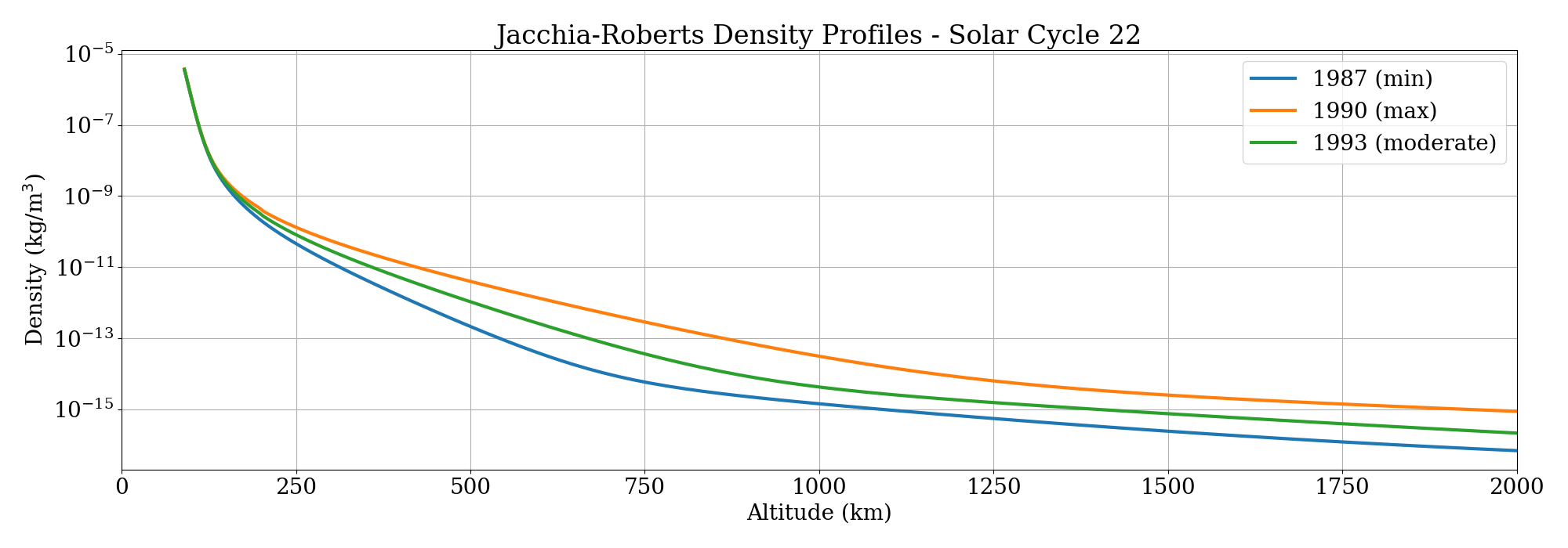
Here's an example output density plot (generated using my pyplot-fortran library) for three epochs near the max/min/average parts of the solar cycle:
Validation
One of the most interesting parts of the process was using AI to help validate the result.
I had no unit tests to start with, but I had two sources of "truth":
- GMAT itself, which I could run to generate density data for different altitudes, epochs, etc. and compare it to the Fortran results.
- An older Fortran implementation of Jacchia-Roberts. This was a Fortran 77 implementation by Valdemir Carrara (Instituto Nacional de Pesquisas Espaciais, INPE) from the 80s, which I obtained from his website, which is no longer there (I archived the codes on GitHub in 2019 thinking I would do something with them one day, and now that day has arrived).
This was also another AI opportunity, since the space weather component of this code was not preserved, so I had Copilot generate a wrapper so that it could call the modern Fortran module we had produced instead.
AI seems to get "unit test happy" sometimes, spewing out numerous long unit tests that do something simple and then prints up elaborate tables with unicode icons and paragraphs of text that tells you what it just tested. That seemed a bit excessive, and I ended up deleting many of the tests it generated, but kept a good number of them. Overall it was quite useful for helping to generate and evaluate tests. When tests failed (e.g., the new results didn't match the other two data sets) I would tell it to investigate to locate the source of the discrepancy, which it could sometimes do successfully, and sometimes not.
The AI went on a flight of fancy for a while trying to figure out a timing discrepancy. It did help me debug it, but it couldn't quite figure it out. At one point I asked if it could go to GitHub and look at the full GMAT code that was there, it told me it could and provided an unconvincing reply suspiciously quickly that it had done so. I guess it was lying to me (Copilot I thought we were friends). I ended up downloading the extra file manually, putting it in the workspace, and directing the AI's attention to it, which seemed to help.
During the validation process, the AI did help me identify three possible issues with the original C++ code. I link the three bug reports I submitted here:
- PrepareKpData uses wrong row index for F10.7a - This is one that the AI detected that I would never have noticed in a million years. It looks like a copy/paste type bug but I'm not 100% sure if it's a real issue or not.
- Legacy UTC calculation used by JacchiaRobertsAtmosphere - This is one that I eventually noticed while trying to debug timing discrepancies during the validation process comparing the results from GMAT to the new version. GMAT (and other GSFC tools) use this crazy alternate definition of modified Julian date (MJD).
So while trying to figure out how to convert what it was outputting in a real MJD, I realized they were using an approximation of UTC (it turns out the correct UTC value output from GMAT is slightly different from what is being used internally by the atmosphere model).
It looks like something that was a holdover from the earlier tools, but I'm not sure if there's a good reason to keep using it.
According to the git history when this file was first committed, the file was originally created for the GSS project in 1995 (I presume this is referring to the Generalized Support Software project at GSFC).
- Low-altitude Jacchia-Roberts bugs - This one is very interesting. There appear to be bugs in the GMAT code for low (<125 km) altitudes. Note that this part of the code is there but not used, since an exception is raised for this case, even though the Jacchia model should support the low altitude ranges (in Roberts' paper, he says his results "are identical" to Jacchia's original equations in the 90 - 125 km altitude regime).
According to the comments and git history on SourceForge, this file was committed in 2004 and the source was the Windows Swingby code (Swingby was another legacy NASA tool that was one of the progenitors of STK/Astrogator).
The
roots function comments says it was converted from existing Fortran code (likely from GTDS, which included the Jacchia-Roberts model).
However, the polynomial deflation technique was written in 1993 based on the "Numerical Recipes in C" book (note that Numerical Recipes talks about the need to "polish" a root found by this method, something not implemented in this code. Maybe that's where they went wrong?)
Is it possible that Swingby had this same bug all those years ago? Or maybe my Fortran conversion is the buggy one? In any event, I replaced this algorithm in the Fortran version with an alternate root finding approach (based on the one in the INPE code) which seems to work fine. I also tested routines from polyroots-fortran and those gave the same results (I might end up just replacing this custom routine with the external dependency).
Legacy Schmegacy

The earlier Fortran tool that some of this code was based on was the Goddard Trajectory Determination System (GTDS). This tool, like many Fortran tools, had a long heritage, but was thrown in the trash in the end, never modernized but replaced with C++ rewrites.
Incidentally, GTDS and Swingby were developed by Computer Sciences Corporation (CSC), a company that existed from 1959 to 2017, which was cofounded by Roy Nutt, one of the members of the original team that created Fortran.
So, now we have come full circle on this wheel of fire with a new modern Fortran port.
Conclusions
The end result of our AI-assisted C++ to Fortran conversion produced something that I think is likely quite useable.
Overall I believe it did save me time compared to how long it would have taken me to do manually. But, getting this over the finish line definitely required manual intervention and domain knowledge.
The process found a few potential bugs in the original code that need to be looked at by actual experts, since I don't trust the AI not a gaslight me with plausible-sounding reasons for them.
Having the AI write the unit tests was also a huge time saver and help with debugging the implementation.
In the end, for a task of this magnitude, I think AI can get you something like 95% of the way there, but then that last 5% needs to be completed and checked very carefully by somebody who more or less knows what they are doing.
Blindly "vibe coding" is dangerous for technical applications such as this, since it's very easy for an AI to provide plausible looking procedures that are totally (or even worse, subtly) wrong.
Note: No AI was used to write the text of this article.
References
- Jacchia, L. G., "New Static Models of the Thermosphere and Exosphere with Empirical Temperature Profiles", Smithsonian Astrophysical Observatory Special Report No. 313, 1970.
- Roberts, C. E., Jr., "An Analytic Model for Upper Atmosphere Densities Based Upon Jacchia's 1970 Models", Celestial Mechanics, Vol. 4, pp. 368-377, 1971.
- GMAT: General Mission Analysis Tool
- Archive of legacy INPE atmosphere models github/@jacobwilliams
- Atmosphere Models [degenerateconic.com] 2021-10-24
- "Does the Programming Language Still Matter When AI Writes Your Code? I Tried Python and Came Back to C#" medium.com/@binnmti, Mar 16, 2026.
- J. Carrico & E. Fletcher, "Software Architecture and Use of Satellite Tool Kit’s Astrogator Module for Libration Point Orbit Missions", Libration Point Orbits and Applications, pp. 471-487 (2003)
- A. C. Long, et al., "Goddard Trajectory Determination System (GTDS) Mathematical Theory Revision 1", FDD/552-89/001, Computer Sciences Corporation, July 1989.
May 10, 2026

Fortran compiler development continues, with regular updates across a range of compilers. Some of the recent updates are summarized below:
Intel
Intel has announced an update to their Fortran compiler (ifx), which is now at version 2026.0.
ifx replaced the venerable ifort compiler a few years ago, and fully supports the Fortran 2018 standard and parts of the Fortran 2023 standard. The Fortran compiler is bundled as part of the Intel's oneAPI Toolkit. According to the release notes, there are only a few updates in this release:
- Support for the leading zero edit mode, which allows a user to control the output of optional leading zeros in numeric outputs.
- A coarray update related to
NOTIFY_TYPE, which I don't understand. Maybe this is useful for somebody. Coarrays are the built-in MPI type feature of Fortran.
- Support for C-style
(a ? b : c) conditional expressions. This was a feature added to Fortran 2023, which is a profoundly weird fit for Fortran syntax, but it does allow a one-line short-circuited logical expression that wasn't otherwise possible before (the merge statement was the closest we had for that before but isn't quite the same).
- Various new OpenMP 6.0 features and a new
-qopenmp-threadprivate option.
- On Windows, support for Microsoft Visual Studio 2026.
Presumably bugs have also been fixed, since the road to ifx adoption has been a little bumpy, with all new bugs that weren't present in ifort. Intel used to call out what bugs were fixed in their compilers, but they haven't done that in years, and users are left to figure out for themselves what might have been fixed.
GFortran
The GNU Project also just released GCC 16.1.
According to the release notes the changes in GFortran are:
- Coarrays using native shared memory multithreading on single node machines and handling Fortran 2018's
TEAM feature.
- Support the Fortran 2018 extensions to the
import statement, the reduce intrinsic and the new generic statement.
- The Fortran 2023 additions to the trigonometric functions are now supported (such as the
sinpi intrinsic).
- The Fortran 2023
split intrinsic subroutine is now supported and c_f_pointer now accepts an optional lower bound as an argument.
- The
-fexternal-blas64 option has been added to call external BLAS routines with 64-bit integer arguments for matmul.
- Parameterized Derived Types (PDT) support is improved. GFortran's implementation of PDT's has been buggy and incomplete for years. PDT was a feature added in Fortran 2003 that looks like it might be useful for writing generic code, but in practice it is not very useful.
Fortran 202y, the next major revision of the Fortran standard is slated to include better generics capabilities.
Honorable mentions
- LFortran also continues to make steady progress towards its first beta release.
- LLVM Flang development also continues, the latest release was 22.1.0. We still don't have Mac builds of this compiler available through conda, so I've never tested this one before. I've gotten this far without having to manually compile a Fortran compiler, and I'm not about to start now.
See also
Apr 26, 2025

The dark ages of confusion about where to get and how to install a Fortran compiler for your platform are over. In recent years, along with the overall renaissance of the Fortran ecosystem, with the conda package manager and the conda-forge package repository, we now have have easy access to all these free compilers for the three major platforms (Windows, Linux, and Mac):
Notes: †† gfortran is the venerable GNU Fortran compiler, the most mature open source Fortran compiler currently available. *ifx is Intel's replacement for ifort using an LLVM backend. It is free but not open source. They did not port it to the Mac ARM architecture, so that version of the compiler does not exist. On Windows, ifx still requires a Visual Studio installation to work.
‡flang (a.k.a. flang-new) is the official LLVM Fortran compiler.
†LFortran, which also uses LLVM, is still under development and is currently an "alpha" product.
There is occasionally hand-wringing from some folks (e.g., SciPy, Los Alamos, etc.) that relying on Fortran compilers is somehow a risky proposition. But it has literally never been easier to install an up-to-date modern compiler for all platforms.
Using conda, installing and trying out a Fortran compiler nowadays is as simple as this:
conda create --prefix ./env gfortran
conda activate ./env
gfortran --version
In addition, a lot of other tools that a Fortran programmer needs nowadays are also available via conda-forge. For example:
- fpm -- Fortran Package Manager
- ford -- Automatically generates Fortran documentation from comments within the code
- fortls -- Fortran Language Server
- fprettify -- Auto-formatter for modern fortran source code
- findent -- Indent, relabel and convert Fortran sources
And you can also find other developer tools you may need including:
- Python (and all the various Python libraries)
- Cmake -- A Powerful Software Build System
- Meson -- Open source build system meant to be both extremely fast, and, even more importantly, as user friendly as possible.
- Ninja -- A small build system with a focus on speed.
- git -- Distributed version control system
So, basically, you can get started with just one command:
conda create --channel conda-forge --prefix ./env gfortran fpm ford fortls fprettify findent cmake meson python git ninja
And it can all be installed in your user directory without requiring admin privileges on the machine (and if you want to remove it just delete that env folder and you are done).
If you are using VSCode, you also will want to install the Modern Fortran extension.
Then from the command palette, you can select "Python: Select Interpreter" and choose the env environment folder you created above. Then you are off to the races.
The conda distribution I recommend is miniforge. This is a version of conda that, by default, uses the conda-forge package channel rather than the commercial Anaconda channels which require a license to use. Note that conda itself is and has always been a free and open source project, so don't let your confused IT department get away with telling you it requires a paid license to use.
Another newer tool is pixi by the folks at prefix.dev. This is billed as a "fast software package manager built on top of the existing conda ecosystem". The syntax and some of the concepts are a little different, but it's an alternative way to install and use conda packages, and also works great.
See also
- Fortran Compilers at fortran-lang.org.
- Navigating Anaconda Licensing Changes: What You Need to Know, Sep 7, 2024.
- LLVM Fortran Levels Up: Goodbye flang-new, Hello flang!, LLVM Project Blog, David Spickett, Mar 11, 2025.
- 7 Reasons to Switch from Conda to Pixi, Wolf Vollprecht, March 1, 2024.
Jan 26, 2025

*From [A FORTRAN Coloring Book](https://archive.org/details/9780262610261) by Roger Kaufman (1978)*
Finding the \(x\) where a scalar function \(f(x) = 0\) is a common problem in numerical programming. There are numerous applications to this. In orbital mechanics, for example, we may want to find the time at which a spacecraft reaches a certain altitude, or enters the Earth's shadow. For these cases, the independent variable is time, and the function \(f\) requires integration of the equations of motion of the spacecraft (for example, by using an IVP solver such as DDEABM). Integrating to an event is often referred to as a "G-stop" feature in these types of applications.
One way to solve this problem is using a derivative-free bracketing method. For these, only function evaluations are used, and the algorithm begins within a set of bounds (\([x_a, x_b]\)) that bracket the root (i.e., \(sign~f(x_a) \ne sign~f(x_b)\)).
Over at the FORTRAN 77 Netlib graveyard, the classic zeroin root finding method can be found that implements such an algorithm, namely Brent's method by Australian mathematician Richard Brent from 1971.

In my roots-fortran library, I have modern Fortran implementations of this method and many others, as well as a lot of benchmark test cases. The library can be compiled for single (real32), double (real64), or quad (real128) precision reals.
For real64 numbers and convergence tolerance \(\epsilon\) = 1.0e-15, the following table lists the number of function evaluations for various methods to converge to the root for various test functions:
| \(f(x)\) |
\([x_a, x_b]\) |
\(x_{root}\) |
BS |
PE |
ITP |
TM |
BR |
AB |
MU |
CH |
| \((x - 1) e^{-x}\) |
\([0,1.5]\) |
1.0 |
46 |
10 |
11 |
9 |
11 |
10 |
9 |
9 |
| \(\cos x - x\) |
\([0,1.7]\) |
0.7390851332151607 |
47 |
8 |
9 |
8 |
8 |
8 |
7 |
8 |
| \(e^{x^2 + 7x - 30} - 1\) |
\([2.6,3.5]\) |
3.0 |
44 |
20 |
17 |
18 |
12 |
31 |
11 |
11 |
| \(x^3\) |
\([-0.5,1/3]\) |
0.0 |
17 |
50 |
16 |
46 |
40 |
38 |
61 |
17 |
| \(x^5\) |
\([-0.5,1/3]\) |
0.0 |
11 |
53 |
12 |
20 |
19 |
39 |
35 |
11 |
| \(\cos x - x^3\) |
\([0,4]\) |
0.8654740331016144 |
48 |
13 |
11 |
13 |
14 |
15 |
10 |
11 |
| \(x^3 - 1\) |
\([0.51,1.5]\) |
1.0 |
46 |
10 |
11 |
9 |
10 |
9 |
7 |
8 |
| \(x^2 ( x^2/3 + \sqrt{2} \sin x ) - \sqrt{3/18}\) |
\([0.1,1]\) |
0.3994222917109682 |
47 |
12 |
17 |
10 |
12 |
12 |
9 |
10 |
| \(x^3 + 1\) |
\([-1.8,0]\) |
-1.0 |
47 |
10 |
10 |
11 |
10 |
12 |
9 |
9 |
| \(\sin((x-7.14)^3)\) |
\([7,8]\) |
7.14 |
18 |
51 |
20 |
48 |
46 |
38 |
52 |
18 |
| \(e^{(x-3)^5} - 1\) |
\([2.6,3.6]\) |
3.0 |
11 |
55 |
12 |
24 |
26 |
41 |
29 |
11 |
| \(e^{(x-3)^5} - e^{x-1}\) |
\([4,5]\) |
4.267168304542125 |
44 |
53 |
45 |
11 |
14 |
58 |
20 |
14 |
| \(\pi - 1/x\) |
\([0.05,5]\) |
\(1 / \pi\) |
50 |
14 |
49 |
18 |
12 |
5 |
13 |
13 |
| \(4 - \tan x\) |
\([0,1.5]\) |
1.325817663668033 |
46 |
14 |
47 |
15 |
13 |
12 |
16 |
15 |
| \(2 x e^{-5} - 2 e^{-5x} + 1\) |
\([0,10]\) |
0.1382571550568241 |
52 |
13 |
16 |
13 |
13 |
11 |
13 |
13 |
The methods are: BS = Bisection, PE = Pegasus, ITP, TM = TOMS 748, BR = Brent, AB = Anderson Bjorck, MU = Muller, and CH = Chandrupatla.
There seems to be cottage industry of creating slight variations of this type of method. There are any number of recent papers on this topic, all claiming some improvement. In reality, a lot of the newer methods really aren't great. An obvious trick is a choose functions where your method behaves well. Another is to only compare against very simple methods (such as bisection or regula falsi, which are known to be inefficient). Finally, the most devious trick is to list the number of iterations of the method, rather than the number of function evaluations, which is basically a useless comparison that obscures the real cost for methods that have multiple function evaluations per iteration.
The Brent method is still one of the best performers. The Chandrupatla method from 1997 is also quite good. For the full set of test cases, see the roots-fortran git repo.
Minimization methods
A related type of algorithm are derivative-free minimization methods. The FMIN function at Netlib is based on Brent's original localmin algorithm (modern version here). The PRIMA library implements modern versions of M.J.D. Powell's derivative-free minimizers for multidimensional functions.
See also
- R. P. Brent, "An algorithm with guaranteed convergence for finding a zero of a function", The Computer Journal, Vol 14, No. 4., 1971.
- R. P. Brent, "Algorithms for Minimization Without Derivatives", Prentice-Hall, 1973.
- Gregory W. Chicares, Brent's method outperforms TOMS 748 [Let me illustrate...]
- T. R. Chandrupatla, "A new hybrid quadratic/bisection algorithm for
finding the zero of a nonlinear function without derivatives", Advances in
Engineering Software, Vol 28, 1997, pp. 145-149.
- M. J. D. Powell, "The BOBYQA algorithm for bound constrained optimization without derivatives," Department of Applied Mathematics and Theoretical Physics, Cambridge England, NA2009/06, 2009.
- polyroots-fortran -- Another modern Fortran library, specifically for finding the roots of polynomials.
Nov 24, 2023

Fortran 2023 (ISO/IEC 1539-1:2023) has been officially published. This replaces the previous standard (Fortran 2018). In a previous post I listed the updates that are in this release (then called "Fortran 202x"). It will be a while before we have fully-compliant Fortran 2023 compilers. In the latest update to the Intel Fortran Compiler, they have started to add a few minor things.
Fortran is the oldest surviving programming language still in common use. Originally developed in 1957, first standardized in 1966, and continuously updated since that time, Fortran remains at the heart of scientific and high-performance computing.
The next standard (unofficially called Fortran 202y) is also already in work.
See also
- Programming languages: Fortran, ISO, Nov. 17, 2023.
- S. Lionel, Fortran 2023 has been Published!, Nov. 23, 2023.
- John Reid, The new features of Fortran 2023, Mar. 13, 2023.
- J. Williams, The New Features of Fortran 202x, Mar 27, 2022.
- Fortran: High-performance parallel programming language
Oct 12, 2022

Image created with the assistance of NightCafe Creator.
Historically, large general-purpose libraries have formed the core of the Fortran scientific ecosystem (e.g., SLATEC, or the various PACKS). Unfortunately, as I have mentioned here before, these libraries were written in FORTRAN 77 (or earlier) and remained unmodified for decades. The amazing algorithms continued within them imprisoned in a terrible format that nobody wants to deal with anymore. At the time they were written, they were state of the art. Now they are relics of the past, a reminder of what might have been if they had continued to be maintained and Fortran had continued to remain the primary scientific and technical programming language.
Over the last few years, I've managed to build up a pretty good set of modern Fortran libraries for technical computing. Some are original, but a lot of them include modernized code from the libraries written decades ago. The codes still work great (polyroots-fortran contains a modernized version of a routine written 50 years ago), but they just needed a little bit of cleanup and polish to be presentable to modern programmers as something other than ancient legacy to be tolerated but not well maintained (which is how Fortran is treated in the SciPy ecosystem).
Here is the list:
| Catagory |
Library |
Description |
Release |
| Interpolation |
bspline-fortran |
1D-6D B-Spline Interpolation |
 |
| Interpolation |
regridpack |
1D-4D linear and cubic interpolation |
 |
| Interpolation |
finterp |
1D-6D Linear Interpolation |
 |
| Interpolation |
PCHIP |
Piecewise Cubic Hermite Interpolation Package |
 |
| Plotting |
pyplot-fortran |
Make plots from Fortran using Matplotlib |
 |
| File I/O |
json-fortran |
Read and write JSON files |
 |
| File I/O |
fortran-csv-module |
Read and write CSV Files |
 |
| Optimization |
slsqp |
SLSQP Optimizer |
 |
| Optimization |
fmin |
Derivative free 1D function minimizer |
 |
| Optimization |
pikaia |
Pikaia Genetic Algorithm |
 |
| Optimization |
simulated-annealing |
Simulated Annealing Algorithm |
 |
| One Dimensional Root-Finding |
roots-fortran |
Roots of continuous scalar functions of a single real variable, using derivative-free methods |
 |
| Polynomial Roots |
polyroots-fortran |
Root finding for real and complex polynomial equations |
 |
| Nonlinear equations |
nlesolver-fortran |
Nonlinear Equation Solver |
 |
| Ordinary Differential Equations |
dop853 |
An explicit Runge-Kutta method of order 8(5,3) |
 |
| Ordinary Differential Equations |
ddeabm |
DDEABM Adams-Bashforth algorithm |
 |
| Numerical Differentiation |
NumDiff |
Numerical differentiation with finite differences |
 |
| Numerical integration |
quadpack |
Modernized QUADPACK Library for 1D numerical quadrature |
 |
| Numerical integration |
quadrature-fortran |
1D-6D Adaptive Gaussian Quadrature |
 |
| Random numbers |
mersenne-twister-fortran |
Mersenne Twister pseudorandom number generator |
 |
| Astrodynamics |
Fortran-Astrodynamics-Toolkit |
Modern Fortran Library for Astrodynamics |
 |
| Astrodynamics |
astro-fortran |
Standard models used in fundamental astronomy |
 |
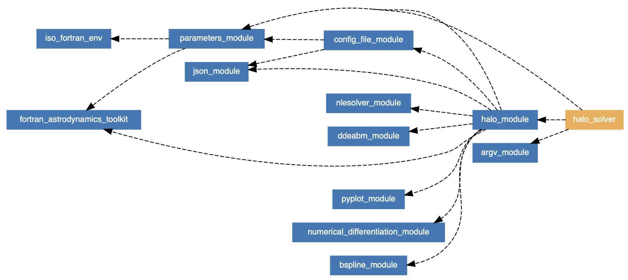
*Example of module dependencies in a Fortran application. This is for the [Halo solver](https://jacobwilliams.github.io/halo/lists/modules.html).*
All of these libraries satisfy my requirements for being part of a modern Fortran scientific ecosystem:
- All are written in a modern Fortran style (free-form, modules, no obsolete constructs such as gotos or common blocks, etc.) All legacy code has been modernized.
- They are all usable with the Fortran Package Manager. A couple of previous posts here and here show how easy it is to do this with a one-line addition to your FPM manifest file.
- The real kind (single, double, or quad precision) is selectable via a preprocessor directive.
- All libraries are available in git repositories on GitHub and contributions are welcome. Every commit is unit tested using GitHub CI.
- All the sourcecode is documented online using FORD.
- All have permissive licenses (e.g., BSD-3) so you can use them however you want.
Fortran has many advantages for scientific computing. It's fast, standard, statically typed, compiled, stable, has a nice array syntax, and includes object oriented programming and native parallelism. It is great for technical and numerical codes that need to run fast and are intended to be used for decades. The libraries listed above will not stop working in a few years. An extremely complicated Fortran application can be recompiled with just a Fortran compiler. You cannot say the same for anything written in the Python scientific ecosystem, which is a Frankenstein hybrid of a scripting language hacked together with a pile of C/C++/Fortran libraries compiled by somebody else. Good luck trying to run Python you write now 20 years from now (or trying to run something written 20 years ago). Fortran is a simple and stable foundation upon which to build our scientific software, Python is not. Having readily available modern libraries along with recent improvements in the Fortran tooling and ecosystem should only serve to make Fortran more appealing in this area.
See also
Jul 31, 2022
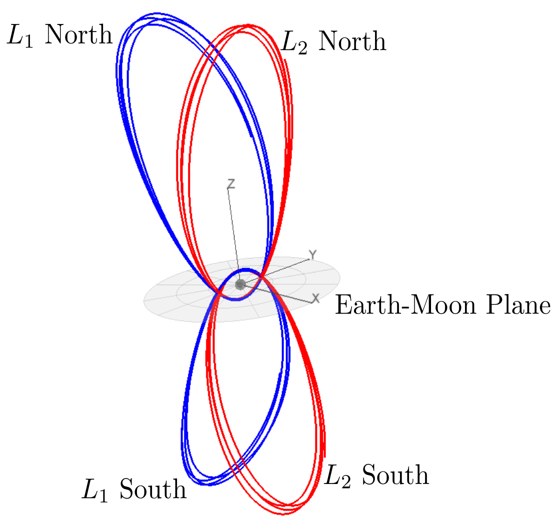
*Some Earth-Moon NRHOs. From [Williams et al, 2017](https://www.researchgate.net/publication/322526659_Targeting_Cislunar_Near_Rectilinear_Halo_Orbits_for_Human_Space_Exploration).*
I have mentioned the Circular Restricted Three-Body Problem (CR3BP) here a couple of times. Another type of periodic CR3BP orbit is the "near rectilinear" halo orbit (NRHO). These orbits are just the continuation of the family of "normal" halo orbits until they get very close to the secondary body [1]. Like all halo orbits, there are "northern" and "southern" families (see image above). NASA chose a lunar L2 NRHO (southern family, which spends more time over the lunar South pole) as the destination orbit for the Deep Space Gateway [2].
The CAPSTONE mission [3] successfully launched on June 28, 2022, and is currently en route to the Gateway NRHO. [4-5]
Computing an NRHO
A basic NRHO in the CR3BP can be computed just like a "normal" halo orbit. (see this and this earlier post). In Reference [2] we described methods for generating long-duration NRHOs in a realistic force model. The procedure involves a multiple shooting method using the CR3BP solution as an initial guess replicated for multiple revs of the orbit. Then a simple nonlinear solver is used to impose state and time continuity for the full orbit.
All we need to start the process is an initial guess. Appendix A.1 in Reference [6] lists a table of CR3BP Earth-Moon L2 halo orbits. An example NRHO from this table is shown here:
| Parameter |
Value |
| \(l^{*}\) |
384400.0 |
| \(t^{*}\) |
375190.25852 |
| Jacobi constant |
3.0411 |
| period |
1.5872714606 |
| \(x_0\) |
1.0277926091 |
| \(z_0\) |
-0.1858044184 |
| \(\dot y_0\) |
-0.1154896637 |
In this table, the three state parameters (\(x_0\), \(z_0\), and \(\dot y_0\)) are given in the canonical normalized CR3BP system, with respect to the Earth-Moon barycenter. The distance and time normalization factors (\(l^{*}\) and \(t^{*}\)) can be used to convert them into normal distance and time units (km and sec).
The process is fairly straightforward, and is demonstrated in a new tool, which I call Halo. It is written in Modern Fortran.
The Halo tool uses the initial CR3BP state to generate a long-duration orbit in the real ephemeris model.
Halo doesn't use the CR3BP equations of motion, since we will be integrating in the real system, using the actual ephemeris of the Earth and Moon, and so we use the real units. See Reference [7] for some further details about an earlier version of this code.
Halo is built upon a number of open source Fortran libraries, and the main components of the tool are:
- General astrodynamics routines, including: ephemeris of the Sun, Earth, and Moon, a spherical harmonic lunar gravity model, state transformations, etc. These are all provided by the Fortran Astrodynamics Toolkit.
- A numerical integration method. I'm using DDEABM, which is an Adams method. I like this method, which has a long heritage and seems to have a good balance of speed and accuracy for these kinds of astrodynamics problems.
- A way to compute derivatives, which are needed by the solver for the Jacobian. For this problem, finite-difference numerical derivatives are good enough, so I'm using my NumDiff library. Since the problem ends up being quite sparse, we can use the NumDiff options to quickly compute the Jacobian matrix by taking into account the sparsity pattern.
- A nonlinear numerical solver. I'm using my nlsolver-fortran library. The problem being solved is "underdetermined", meaning there are more free variables than there are constraints. Nlsolver-Fortran can solve these problems just fine using a basic Newton-type minimum norm method. In astrodynamics, you will usually see this type of method called a "differential corrector".
Halo makes use of the amazing Fortran Package Manager (FPM) for dependency management and compilation. In the fpm.toml manifest file, all we have to do is specify the dependencies like so:
[dependencies]
fortran-astrodynamics-toolkit = { git = "https://github.com/jacobwilliams/Fortran-Astrodynamics-Toolkit", tag = "0.4" }
NumDiff = { git = "https://github.com/jacobwilliams/NumDiff", tag = "1.5.1" }
ddeabm = { git = "https://github.com/jacobwilliams/ddeabm", tag = "3.0.0" }
json-fortran = { git = "https://github.com/jacobwilliams/json-fortran", tag = "8.2.5" }
bspline-fortran = { git = "https://github.com/jacobwilliams/bspline-fortran", tag = "6.1.0" }
pyplot-fortran = { git = "https://github.com/jacobwilliams/pyplot-fortran", tag = "3.2.0" }
fortran-search-and-sort = { git = "https://github.com/jacobwilliams/fortran-search-and-sort", tag = "1.0.0" }
fortran-csv-module = { git = "https://github.com/jacobwilliams/fortran-csv-module", tag = "1.3.0" }
nlesolver-fortran = { git = "https://github.com/jacobwilliams/nlesolver-fortran", tag = "1.0.0" }
argv-fortran = { git = "https://github.com/jacobwilliams/argv-fortran", tag = "1.0.0" }
FPM will download the specified versions of everything and build the tool with a single command like so:
fpm build --profile release
This is really a game changer for Fortran. Before FPM, poor Fortran users had no package manager at all. A common anti-pattern was to manually download code from somewhere like Netlib and then manually add the files to your repo and manually edit your makefiles to incorporate it into your compile process. This is literally what SciPy has done, and now they have forks of all their Fortran code that just lives inside the SciPy monorepo, with no way to distribute it upstream to the original library source, or downstream to other Fortran codes that might want to use it. FPM makes it all just effortless to specify dependencies (and update the version numbers if the upstream code changes) and finally allows and encourages Fortran users to develop a modern system of interdependent libraries with sane and modern version control practices.
Example
Using the initial guess from the table above, we can use Halo to compute a ballistic NRHO for 50 revs (about 344 days for this example) in the real ephemeris model. The 50 rev problem has 1407 control variables and 1200 equality constraints. Convergence takes about 31 seconds (6 iterations of the solver) on my M1 MacBook Pro, complied using the Intel Fortran compiler:
| Iteration number |
norm2(Constraint violation vector) |
| 1 |
0.2936000870578949 |
| 2 |
0.1554308242228055 |
| 3 |
0.0611200979653433 |
| 4 |
0.0052758762761737 |
| 5 |
0.0000031933098398 |
| 6 |
0.0000000035186120 |
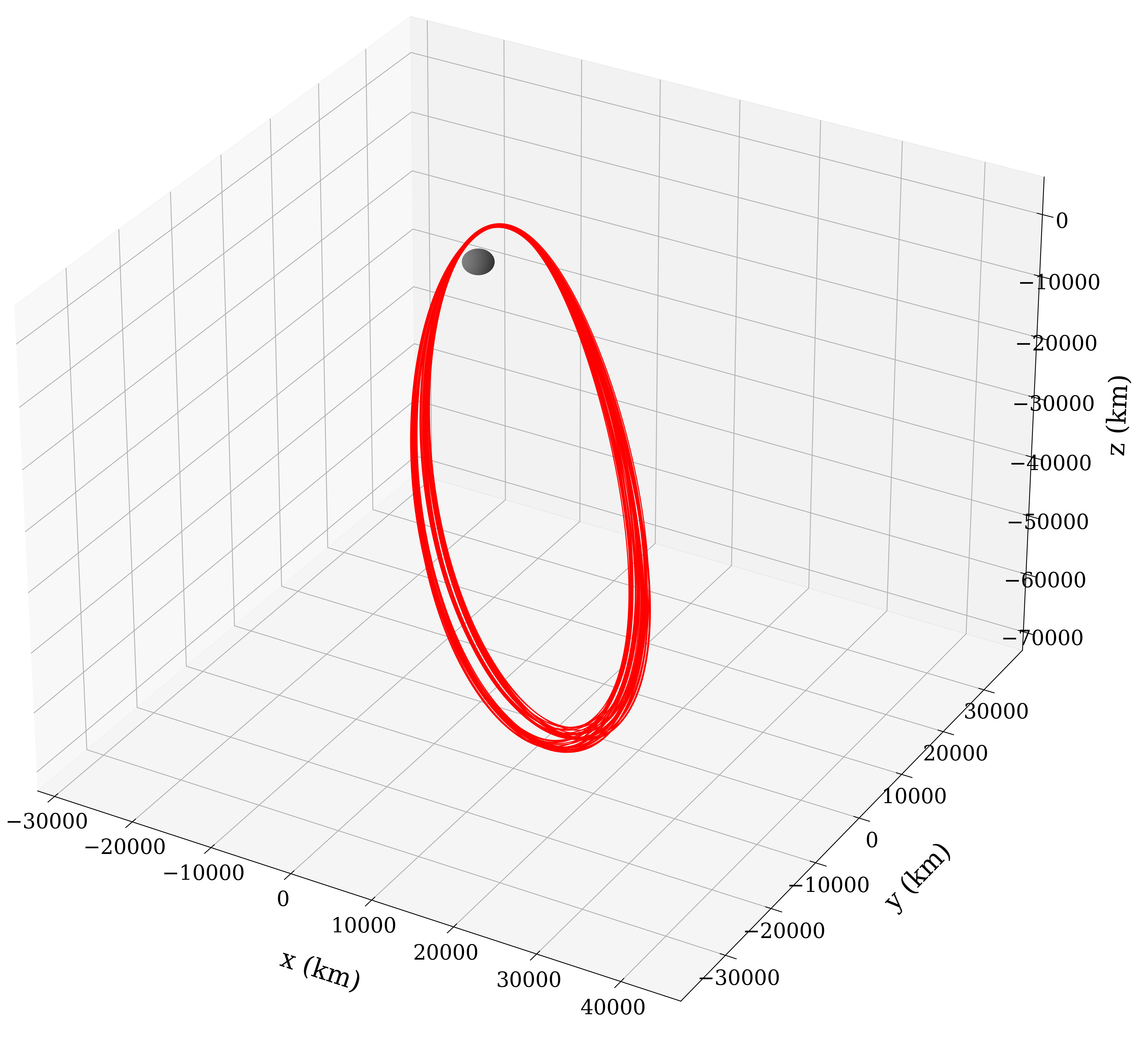
*50 Rev NRHO Solution. Visualized here in the Moon-centered Earth-Moon rotating frame.*
There's no parallelization currently being used here, so there are some opportunities to speed it up even more.
In Reference [2] we also show how the above procedure can be used to kick off a "receding horizon" approach to compute even longer duration NRHOs that include very small correction burns. This is the process that was used to generate the Gateway orbit [4-5], and the Halo program could be updated to do that as well. But that is a post for another time.
See also
- K. C. Howell & J. V. Breakwell, "Almost rectilinear halo orbits", Celestial mechanics volume 32, pages 29--52 (1984)
- J. Williams, D. E. Lee, R. J. Whitley, K. A. Bokelmann, D. C. Davis, and C. F. Berry. "Targeting cislunar near rectilinear halo orbits for human space exploration", AAS 17-267
- What is CAPSTONE?, NASA, Apr 29, 2022
- D. E. Lee, "Gateway Destination Orbit Model: A Continuous 15 Year NRHO Reference Trajectory", August 20, 2019
- D. E. Lee, R. J. Whitley and C. Acton, "Sample Deep Space Gateway Orbit, NAIF Planetary Data System Navigation Node", NASA Jet Propulsion Laboratory, July 2018.
- E. M. Z. Spreen, "Trajectory Design and Targeting For Applications to the Exploration Program in Cislunar Space", PhD Dissertation, Purdue University, 2021
- J. Williams, R. D. Falck, and I. B. Beekman, "Application of Modern Fortran to Spacecraft Trajectory Design and Optimization", 2018 Space Flight Mechanics Meeting, 8–12 January 2018, AIAA 2018-145.


