Jun 19, 2022

[NightCafe](https://creator.nightcafe.studio/) AI generated image for "old computers"
The classic Fortran routines r1mach (for single precision real numbers), d1mach (for double precision real numbers), and i1mach (for integers) were originally written in the mid-1970s for the purpose of returning basic machine or operating system dependent constants in order to provide portability. Typically, these routines had a bunch of commented out DATA statements, and the user was required to uncomment out the ones for their specific machine. The original versions included constants for the following systems:
Over the years, various versions of these routines have been created:
In the Fortran 90 versions, the original routines were modified to use various intrinsic functions available in Fortran 90. However, some hard-coded values remained in i1mach. With the advent of more recent standards, it is now possible to provide modern and completely portable versions which are described below. Starting with the Fortran 90 versions, the following changes were made:
- The routines are now in a module. We declare two module parameters which will be used in the routines:
integer, parameter :: sp = kind(1.0)    ! single precision kind
integer, parameter :: dp = kind(1.0d0)  ! double precision kind
Of course, putting them in a module means that they are not quite drop-in replacements for the old routines. If you want to use this module with legacy code, you'd have to update your code to add a use statement. But that's the way it goes. Nobody should be writing Fortran anymore that isn't in a module, so I'm not going to encourage that.
-
The comment strings have been updated to Ford-style. I find the old SLATEC comment block style extremely cluttered. Various cosmetic changes were also made (e.g., changing the old .GE. to >=, etc.)
-
All three routines were made pure. The error stop construct was used for the out of bounds input condition (Fortran 2008 allows error stop in pure procedures).
-
New intrinsic constants available in the Fortran 2008 standard were employed (see below).
The new routines can be found on GitHub. They are shown below without the comment blocks.
The new routines
The new d1mach routine is:
D1MACH
  pure real(dp) function d1mach(i)

    integer, intent(in) :: i

    real(dp), parameter :: x = 1.0_dp
    real(dp), parameter :: b = real(radix(x), dp)

    select case (i)
    case (1); d1mach = b**(minexponent(x) - 1) ! the smallest positive magnitude.
    case (2); d1mach = huge(x)                 ! the largest magnitude.
    case (3); d1mach = b**(-digits(x))         ! the smallest relative spacing.
    case (4); d1mach = b**(1 - digits(x))      ! the largest relative spacing.
    case (5); d1mach = log10(b)
    case default
        error stop 'Error in d1mach - i out of bounds'
    end select

  end function d1mach
This is mostly just a reformatting of the Fortran 90 routine. We make x and b parameters, and use error stop for the error condition rather than this monstrosity:
          WRITE (*, FMT = 9000)
 9000     FORMAT ('1ERROR    1 IN D1MACH - I OUT OF BOUNDS')
          STOP
R1MACH
The updated R1MACH is similar, except the real values are real(sp) (default real, or single precision):
  pure real(sp) function r1mach(i)

    integer, intent(in) :: i

    real(sp), parameter :: x = 1.0_sp
    real(sp), parameter :: b = real(radix(x), sp)

    select case (i)
    case (1); r1mach = b**(minexponent(x) - 1) ! the smallest positive magnitude.
    case (2); r1mach = huge(x)                 ! the largest magnitude.
    case (3); r1mach = b**(-digits(x))         ! the smallest relative spacing.
    case (4); r1mach = b**(1 - digits(x))      ! the largest relative spacing.
    case (5); r1mach = log10(b)
    case default
      error stop 'Error in r1mach - i out of bounds'
    end select

  end function r1mach
I1MACH
The new i1mach routine is:
  pure integer function i1mach(i)

    integer, intent(in) :: i

    real(sp), parameter :: x = 1.0_sp
    real(dp), parameter :: xx = 1.0_dp

    select case (i)
    case (1);  i1mach = input_unit
    case (2);  i1mach = output_unit
    case (3);  i1mach = 0  ! Punch unit is no longer used
    case (4);  i1mach = error_unit
    case (5);  i1mach = numeric_storage_size
    case (6);  i1mach = numeric_storage_size / character_storage_size
    case (7);  i1mach = radix(1)
    case (8);  i1mach = numeric_storage_size - 1
    case (9);  i1mach = huge(1)
    case (10); i1mach = radix(x)
    case (11); i1mach = digits(x)
    case (12); i1mach = minexponent(x)
    case (13); i1mach = maxexponent(x)
    case (14); i1mach = digits(xx)
    case (15); i1mach = minexponent(xx)
    case (16); i1mach = maxexponent(xx)
    case default
      error stop 'Error in i1mach - i out of bounds'
    end select

  end function i1mach
In this one, we make heavy use of constants now in the intrinsic iso_fortran_env module, including input_unit, output_unit, error_unit, numeric_storage_size, and character_storage_size. In the Fortran 90 code, the values for I1MACH(1:4) and I1MACH(6) were totally not portable. This new one is now (almost) entirely portable.
The only remaining parameter that cannot be expressed portably is I1MACH(3), the standard punch unit. If you look at the original i1mach.f from SLATEC, there were a range of values of this parameter used by various machines (e.g. 102 for the Cray, or 7 for the IBM 360/370). Hopefully, this is not something that anybody needs nowadays, so we leave it set to 0 in the updated routine. If the Fortran committee ever adds punch_unit to iso_fortran_env, then we can update it then, and this routine will finally be finished, and the promise of a totally portable machine constants routine will finally be fulfilled.
Another interesting thing to note are I1MACH(7) (which is RADIX(1)) and I1MACH(10) (which is RADIX(1.0)). There was no I1MACH parameter for RADIX(1.0D0).
There were machine architectures where I1MACH(7) /= I1MACH(10). For example, the Data General Eclipse S/200 had I1MACH(7)=2 and I1MACH(10)=16.
But, it seems unlikely that there would ever be an architecture where the radix would be different for different real kinds. So maybe we are safe?
Results
On my laptop (Apple M1) with gfortran, the three routines produce the following values:
i1mach( 1) =                5
i1mach( 2) =                6
i1mach( 3) =                0
i1mach( 4) =                0
i1mach( 5) =               32
i1mach( 6) =                4
i1mach( 7) =                2
i1mach( 8) =               31
i1mach( 9) =       2147483647
i1mach(10) =                2
i1mach(11) =               24
i1mach(12) =             -125
i1mach(13) =              128
i1mach(14) =               53
i1mach(15) =            -1021
i1mach(16) =             1024

r1mach( 1) =             1.17549435E-038    (            800000 )
r1mach( 2) =             3.40282347E+038    (          7F7FFFFF )
r1mach( 3) =             5.96046448E-008    (          33800000 )
r1mach( 4) =             1.19209290E-007    (          34000000 )
r1mach( 5) =             3.01030010E-001    (          3E9A209B )

d1mach( 1) =   2.22507385850720138E-0308    (    10000000000000 )
d1mach( 2) =   1.79769313486231571E+0308    (  7FEFFFFFFFFFFFFF )
d1mach( 3) =   1.11022302462515654E-0016    (  3CA0000000000000 )
d1mach( 4) =   2.22044604925031308E-0016    (  3CB0000000000000 )
d1mach( 5) =   3.01029995663981198E-0001    (  3FD34413509F79FF )
References
- P. A. Fox, A. D. Hall and N. L. Schryer, Algorithm 528: Framework for a portable library, ACM Transactions on Mathematical Software 4, 2 (June 1978), pp. 177-188.
- David Gay and Eric Grosse, Self-Adapting Fortran 77 Machine Constants: Comment on Algorithm 528, ACM Transactions on Mathematical Software 25, 1 (March 1999), pp. 123-126.
- Bo Einarsson, d1mach revisited: no more uncommenting DATA statements Presented at the IFIP WG 2.5 International Workshop on "Current Directions in Numerical Software and High Performance Computing", 19 - 20 October 1995, Kyoto, Japan.
- An interview with Phyllis A. Fox, Conducted by Thomas Haigh on 7 and 8 June, 2005, Short Hills, New Jersey. Interview conducted by the Society for Industrial and Applied Mathematics.
- Why no punch_unit in iso_fortran_env?, Jun 18, 2022 [Fortran-lang Discourse]
Jun 17, 2022

In today's episode of "What where the Fortran dudes in the 1980s thinking?": consider the following code, which can be found in various forms in the two SLATEC quadrature routines dgaus8 and dqnc79:
K = I1MACH(14)
ANIB = D1MACH(5)*K/0.30102000D0
NBITS = ANIB
Note that the "mach" routines (more on that below) return:
I1MACH(10) = B, the base. This is equal to 2 on modern hardware.I1MACH(14) = T, the number of base-B digits for double precision. This will be 53 on modern hardware.D1MACH(5) = LOG10(B), the common logarithm of the base.
First off, consider the 0.30102000D0 magic number. Is this supposed to be log10(2.0d0) (which is 0.30102999566398120)? Is this a 40 year old typo? It looks like they ended it with 2000 when they meant to type 3000? In single precision, log10(2.0) is 0.30103001. Was it just rounded wrong and then somebody added a D0 to it at some point when they converted the routine to double precision? Or is there some deep reason to make this value very slightly less than log10(2.0)?
But it turns out, there is a reason!
If you look at the I1MACH routine from SLATEC you will see constants for computer hardware from the dawn of time (well, at least back to 1975. It was last modified in 1993). The idea was you were supposed to uncomment the one for the hardware you were running on. Remember how I said IMACH(10) was equal to 2? Well, that was not always true. For example, there was something called a Data General Eclipse S/200, where IMACH(10) = 16 and IMACH(14) = 14. Who knew?
So, if we compare two ways to do this (in both single and double precision):
! slatec way:
 anib_real32  = log10(real(b,real32))*k/0.30102000_real32;   nbits_real32  = anib_real32
 anib_real64  = log10(real(b,real64))*k/0.30102000_real64;   nbits_real64  = anib_real64

! naive way:
 anib_real32_alt  = log10(real(b,real32))*k/log10(2.0_real32);   nbits_real32_alt  = anib_real32_alt
 anib_real64_alt  = log10(real(b,real64))*k/log10(2.0_real64);   nbits_real64_alt  = anib_real64_alt

! note that k = imach(11) for real32, and imach14 for real64
We see that, for the following architectures from the i1mach routine, the naive way will give the wrong answer:
- BURROUGHS 5700 SYSTEM (real32: 38 instead of 39, and real64: 77 instead of 78)
- BURROUGHS 6700/7700 SYSTEMS (real32: 38 instead of 39, and real64: 77 instead of 78)
The reason is because of numerical issues and the fact that the real to integer assignment will round down. For example, if the result is 38.99999999, then that will be rounded down to 38. So, the original programmer divided by a value slightly less than log10(2) so the rounding would come out right. Now, why didn't they just use a rounding function like ANINT? Apparently, that was only added in Fortran 77. Work on SLATEC began in 1977, so likely they started with Fortran 66 compilers. And so this bit of code was never changed and we are still using it 40 years later.
Numeric inquiry functions
In spite of most or all of the interesting hardware options of the distant past no longer existing, Fortran is ready for them, just in case they come back! The standard includes a set of what are called numeric inquiry functions that can be used to get these values for different real and integer kinds:
| Name |
Description |
| BIT_SIZE |
The number of bits in an integer type |
| DIGITS |
The number of significant digits in an integer or real type |
| EPSILON |
Smallest number that can be represented by a real type |
| HUGE |
Largest number that can be represented by a real type |
| MAXEXPONENT |
Maximum exponent of a real type |
| MINEXPONENT |
Minimum exponent of a real type |
| PRECISION |
Decimal precision of a real type |
| RADIX |
Base of the model for an integer or real type |
| RANGE |
Decimal exponent range of an integer or real type |
| TINY |
Smallest positive number that can be represented by a real type |
So, the D1MACH and I1MACH routines are totally unnecessary nowadays. Modern versions that are simply wrappers to the intrinsic functions can be found here, which may be useful for backward compatibility purposes when using old codes. I tend to just replace calls to these functions with calls to the intrinsic ones when I have need to modernize old code.
Updating the old code
In modern times, we can replace the mysterious NBITS code with the following (maybe) slightly less mysterious version:
 integer,parameter :: nbits = anint(log10(real(radix(1.0_wp),wp))*digits(1.0_wp)/log10(2.0_wp))

 ! on modern hardware, nbits is: 24 for real32
 !                               53 for real64
 !                              113 for real128
Where:
wp is the real precision we want (e.g., real32 for single precision, real64 for double precision, and real128 for quad precision).radix(1.0_wp) is equivalent to the old I1MACH(10)digits(1.0_wp) is equivalent ot the old I1MACH(14)
Thus we don't need the "magic" number anymore, so it's time to retire it. I plan to make this change in the refactored Quadpack library, where these routines are being cleaned up and modernized in order to serve for another 40 years. Note that, for modern systems, this equation reduces to just digits(1.0_wp), but I will keep the full equation, just in case. It will even work on the Burroughs, just in case those come back in style.

Final thought
If you search the web for "0.30102000" you can find various translations of these old quadrature routines. My favorite is this Java one:
//  K = I1MACH(14) --- SLATEC's i1mach(14) is the number of base 2
//  digits for double precision on the machine in question.  For
//  IEEE 754 double precision numbers this is 53.

      k = 53;

//  r1mach(5) is the log base 10 of 2 = .3010299957

//      anib = .3010299957*k/0.30102000E0;

//      nbits = (int)(anib);

      nbits = 53;
Great job guys!
Acknowlegments
Special thanks to Fortran-lang Discourse users @urbanjost, @mecej4, and @RonShepard in this post for helping me get to the bottom of the mysteries of this code.
See also
- P. A. Fox, A. D. Hall and N. L. Schryer, Framework for a portable library, ACM Transactions on Mathematical Software 4, 2 (June 1978), pp. 177-188.
- David Gay and Eric Grosse, d1mach revisited: no more uncommenting DATA statements, Presented at the IFIP WG 2.5 International Workshop on "Current Directions in Numerical Software and High Performance Computing", 19 - 20 October 1995, Kyoto, Japan.
- Fun with 40 year old code, June 11, 2022, [fortran-lang Discourse].
- SLATEC, May 15, 2016 [degenerateconic.com]
- Quadpack -- Modern Fortran QUADPACK Library for 1D numerical quadrature [GitHub]
- Sorting with Magic Numbers, July 5, 2014 [degenerateconic.com]
- Burroughs large systems [Wikipedia]
May 15, 2016
The SLATEC Common Mathematical Library (CML) is written in FORTRAN 77 and contains over 1400 general purpose mathematical and statistical routines. SLATEC is an acronym for the "Sandia, Los Alamos, Air Force Weapons Laboratory Technical Exchange Committee", an organization formed in 1974 by the computer centers of these organizations. In 1977, it was decided to build a FORTRAN library to provide portable, non-proprietary, mathematical software for member sites' supercomputers. Version 1.0 of the CML was released in April 1982.
An example SLATEC routine is shown below, which computes the inverse hyperbolic cosine:
*DECK ACOSH
    FUNCTION ACOSH (X)
C***BEGIN PROLOGUE ACOSH
C***PURPOSE Compute the arc hyperbolic cosine.
C***LIBRARY SLATEC (FNLIB)
C***CATEGORY C4C
C***TYPE SINGLE PRECISION (ACOSH-S, DACOSH-D, CACOSH-C)
C***KEYWORDS ACOSH, ARC HYPERBOLIC COSINE, ELEMENTARY FUNCTIONS, FNLIB,
C INVERSE HYPERBOLIC COSINE
C***AUTHOR Fullerton, W., (LANL)
C***DESCRIPTION
C
C ACOSH(X) computes the arc hyperbolic cosine of X.
C
C***REFERENCES (NONE)
C***ROUTINES CALLED R1MACH, XERMSG
C***REVISION HISTORY (YYMMDD)
C 770401 DATE WRITTEN
C 890531 Changed all specific intrinsics to generic. (WRB)
C 890531 REVISION DATE from Version 3.2
C 891214 Prologue converted to Version 4.0 format. (BAB)
C 900315 CALLs to XERROR changed to CALLs to XERMSG. (THJ)
C 900326 Removed duplicate information from DESCRIPTION section.
C (WRB)
C***END PROLOGUE ACOSH
    SAVE ALN2,XMAX
    DATA ALN2 / 0.6931471805 5994530942E0/
    DATA XMAX /0./
C***FIRST EXECUTABLE STATEMENT ACOSH
    IF (XMAX.EQ.0.) XMAX = 1.0/SQRT(R1MACH(3))
C
    IF (X .LT. 1.0) CALL XERMSG ('SLATEC', 'ACOSH', 'X LESS THAN 1',
  + 1, 2)
C
    IF (X.LT.XMAX) ACOSH = LOG (X + SQRT(X*X-1.0))
    IF (X.GE.XMAX) ACOSH = ALN2 + LOG(X)
C
    RETURN
    END
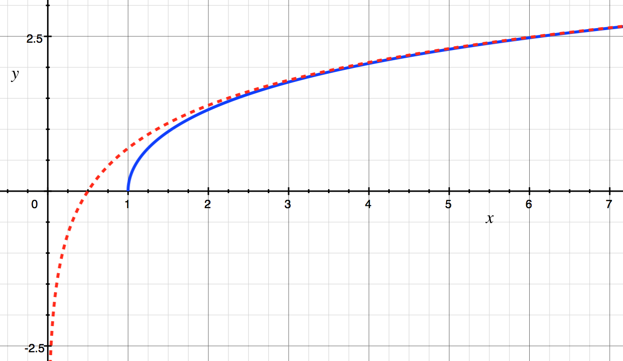
Of course, this routine is full of nonsense from the point of view of a modern Fortran programmer (fixed-form source, implicitly typed variables, SAVE and DATA statements, constants computed at run time rather than compile time, hard-coding of the numeric value of ln(2), etc.). And you don't even want to know what's happening in the R1MACH() function. A modern version would look something like this:
pure elemental function acosh(x) result(acoshx)

!! arc hyperbolic cosine

use iso_fortran_env, only: wp => real64

implicit none

real(wp),intent(in) :: x
real(wp) :: acoshx

real(wp),parameter :: aln2 = &
    log(2.0_wp)
real(wp),parameter :: r1mach3 = &
    real(radix(1.0_wp),wp)**(-digits(1.0_wp)) !! largest relative spacing
real(wp),parameter :: xmax = &
    1.0_wp/sqrt(r1mach3)

if ( x<1.0_wp ) then
    error stop 'slatec : acosh : x less than 1'
else
    if ( x<xmax ) then
        acoshx = log(x + sqrt(x*x - 1.0_wp))
    else
        acoshx = aln2 + log(x)
    end if
end if

end function acosh
Of course, the point is moot, since ACOSH() is now an intrinsic function in Fortran 2008, so we don't need either of these anymore. Unfortunately, like many great Fortran codes, SLATEC has been frozen in amber since the early 1990's. It does contain a great many gems, however, and any deficiencies in the original Fortran 77 code can be easily remedied using modern Fortran standards. See also, for example, my own DDEABM project, which is a complete refactoring and upgrade of the Adams-Bashforth-Moulton ODE solver from SLATEC.
The GNU Scientific Library was started in 1996 to be a "modern version of SLATEC". Of course, rather than refactoring into modern Fortran (Fortran 90 had been published several years earlier, but I believe it was some time before a free compiler was available) they decided to start over in C. There's now even a Fortran interface to GSL (so now we can use a Fortran wrapper to call a C function that replaced a Fortran function that worked perfectly well to begin with!) The original SLATEC was a public domain work of the US government, and so can be used without restrictions in free or proprietary applications, but GSL is of course, GPL, so you're out of luck if you are unable to accept the ~~restrictions~~ (I mean freedom) of that license.
Note that John Burkardt has produced a version of SLATEC translated to free-form source. The license for this modified version is unclear. Many of his other codes are LGPL (still more restrictive than the original public domain codes). It's not a full refactoring, either. The codes still contain non-standard extensions and obsolescent and now-unnecessary features such as COMMON blocks. What we really need is a full modern refactoring of SLATEC (and other unmaintained codes like the NIST CMLIB and NSWC, etc.)
References
- Fong, Kirby W., Jefferson, Thomas H., Suyehiro, Tokihiko, Walton, Lee, "Guide to the SLATEC Common Mathematical Library", July 1993.
- SLATEC source code at Netlib.
Dec 28, 2015
DDEABM is variable step size, variable order Adams-Bashforth-Moulton PECE solver for integrating a system of first order ordinary differential equations [1-2]. It is a public-domain code originally developed in the 1970s-1980s, written in FORTRAN 77, and is available from Netlib (as part of the SLATEC Common Mathematical Library). DDEABM is primarily designed to solve non-stiff and mildly-stiff differential equations when derivative evaluations are expensive, high accuracy results are needed or answers at many specific points are required. It is based on the earlier ODE/STEP/INTRP codes described in [3-4].
DDEABM is a great code, but like many of the greats of Fortran, it seems to have been frozen in amber for 30 years. There are a couple of translations into other programming languages out there such as IDL and Matlab. It is also the ancestor of the Matlab ode113 solver (indeed, they were both written by the same person [5]). But, it looks like poor Fortran users have been satisfied with using it as is, in all its FORTRAN 77 glory.
So, I've taken the code and significantly refactored it to bring it up to date to modern standards (Fortran 2003/2008). This is more than just a conversion from fixed to free-form source. The updated version is now object-oriented and thread-safe, and also has a new event finding capability (there is a version of this code that had root-finding capability, but it seems to be based on an earlier version of the code, and also has some limitations such as a specified maximum number of equations). The new event finding feature incorporates the well-known ZEROIN algorithm [6-7] for finding a root on a bracketed interval. Everything is wrapped up in an easy-to-use class, and it also supports the exporting of intermediate integration points.
The new code is available on GitHub and is released under a permissive BSD-style license. It is hoped that it will be useful. There are some other great ODE codes that could use the same treatment (e.g. DLSODE/DVODE from ODEPACK, DIVA from MATH77, and DOP853 from Ernst Hairer).
References
- L. F. Shampine, H. A. Watts, "DEPAC - Design of a user oriented package of ode solvers", Report SAND79-2374, Sandia Laboratories, 1979.
- H. A. Watts, "A smoother interpolant for DE/STEP, INTRP and DEABM: II", Report SAND84-0293, Sandia Laboratories, 1984.
- L. F. Shampine, M. K. Gordon, "Solving ordinary differential equations with ODE, STEP, and INTRP", Report SLA-73-1060, Sandia Laboratories, 1973.
- L. F. Shampine, M. K. Gordon, "Computer solution of ordinary differential equations, the initial value problem", W. H. Freeman and Company, 1975.
- L. F. Shampine and M. W. Reichelt, "The MATLAB ODE Suite" [MathWorks].
- R. P. Brent, "An algorithm with guaranteed convergence for finding a zero of a function", The Computer Journal, Vol 14, No. 4., 1971.
- R. P. Brent, "Algorithms for minimization without derivatives", Prentice-Hall, Inc., 1973.
Jul 05, 2014
Updated July 7, 2014
Poorly commented sourcecode is one of my biggest pet peeves. Not only should the comments explain what the routine does, but where the algorithm came from and what its limitations are. Consider ISORT, a non-recursive quicksort routine from SLATEC, written in 1976. In it, we encounter the following code:
R = 0.375E0
...
IF (R .LE. 0.5898437E0) THEN
    R = R+3.90625E-2
ELSE
    R = R-0.21875E0
ENDIF
What are these magic numbers? An internet search for "0.5898437" yields dozens of hits, many of them different versions of this algorithm translated into various other programming languages (including C, C++, and free-format Fortran). Note: the algorithm here is the same one, but also prefaces this code with the following helpful comment:
! And now...Just a little black magic...
Frequently, old code originally written in single precision can be improved on modern computers by updating to full-precision constants (replacing 3.14159 with a parameter computed at compile time as acos(-1.0_wp) is a classic example). Is this the case here? Sometimes WolframAlpha is useful in these circumstances. It tells me that a possible closed form of 0.5898437 is: \(\frac{57}{100\pi}+\frac{13\pi}{100} \approx 0.58984368009\). Hmmmmm... The reference given in the header is no help [1], it doesn't contain this bit of code at all.
It turns out, what this code is doing is generating a pseudorandom number to use as the pivot element in the quicksort algorithm. The code produces the following repeating sequence of values for R:
0.375
0.4140625
0.453125
0.4921875
0.53125
0.5703125
0.609375
0.390625
0.4296875
0.46875
0.5078125
0.546875
0.5859375
0.625
0.40625
0.4453125
0.484375
0.5234375
0.5625
0.6015625
0.3828125
0.421875
0.4609375
0.5
0.5390625
0.578125
0.6171875
0.3984375
0.4375
0.4765625
0.515625
0.5546875
0.59375
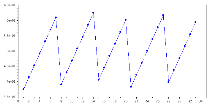
This places the pivot point near the middle of the set. The source of this scheme is from Reference [2], and is also mentioned in Reference [3]. According to [2]:
These four decimal constants, which are respectively 48/128, 75.5/128, 28/128, and 5/128, are rather arbitrary.
The other magic numbers in this routine are the dimensions of these variables:
These are workspace arrays used by the subroutine, since it does not employ recursion. But, since they have a fixed size, there is a limit to the size of the input array this routine can sort. What is that limit? You would not know from the documentation in this code. You have to go back to the original reference [1] (where, in fact, these arrays only had 16 elements). There, it explains that the arrays IL(K) and IU(K) permit sorting up to \(2^{k+1}-1\) elements (131,071 elements for the k=16 case). With k=21, that means the ISORT routine will work for up to 4,194,303 elements. So, keep that in mind if you are using this routine.
There are many other implementations of the quicksort algorithm (which was declared one of the top 10 algorithms of the 20th century). In the LAPACK quicksort routine DLASRT, k=32 and the "median of three" method is used to select the pivot. The quicksort method in R is the same algorithm as ISORT, except that k=40 (this code also has the advantage of being properly documented, unlike the other two).
References
- R. C. Singleton, "Algorithm 347: An Efficient Algorithm for Sorting With Minimal Storage", Communications of the ACM, Vol. 12, No. 3 (1969).
- R. Peto, "Remark on Algorithm 347", Communications of the ACM, Vol. 13 No. 10 (1970).
- R. Loeser, "Survey on Algorithms 347, 426, and Quicksort", ACM Transactions on Mathematical Software (TOMS), Vol. 2 No. 3 (1976).