Polynomial Roots
Consider the problem of finding all the roots of a polynomial. This involves solving the following equation:
This problem occurs in many different applications, such as computing atmospheric density in a spacecraft orbit simulation. In general, both the coefficients and roots can be complex numbers. A special case involves only real coefficients. General methods exist for any degree polynomial, and custom methods also exist for polynomials of specific degree. The quadratic formula is the most famous analytical solution for polynomials of degree 2. In general, numerical methods are necessary to solve polynomials of degree 5 and higher.
Newton's method is frequently used, which requires an initial guess and an iterative procedure. Another elegant way to solve for all the roots at once is to find the eigenvalues of the companion matrix.
Fortran library

My polyroots-fortran library includes various methods to solve this problem. Many of the implementations have legacy going back decades (for example, from SLATEC). It's easy to incorporate into other codes using the Fortran Package Manager. The available methods in the library are:
| Method name | Polynomial type | Coefficients | Reference |
|---|---|---|---|
cpoly |
General | complex | Jenkins & Traub (1972) |
rpoly |
General | real | Jenkins & Traub (1975) |
rpzero |
General | real | SLATEC |
cpzero |
General | complex | SLATEC |
rpqr79 |
General | real | SLATEC |
cpqr79 |
General | complex | SLATEC |
dqtcrt |
Quartic | real | NSWC Library |
dcbcrt |
Cubic | real | NSWC Library |
dqdcrt |
Quadratic | real | NSWC Library |
quadpl |
Quadratic | real | NSWC Library |
dpolz |
General | real | MATH77 Library |
cpolz |
General | complex | MATH77 Library |
polyroots |
General | real | LAPACK |
cpolyroots |
General | complex | LAPACK |
rroots_chebyshev_cubic |
Cubic | real | Lebedev (1991) |
qr_algeq_solver |
General | real | Edelman & Murakami (1995) |
polzeros |
General | complex | Bini (1996) |
cmplx_roots_gen |
General | complex | Skowron & Gould (2012) |
fpml |
General | complex | Cameron (2019) |
Example
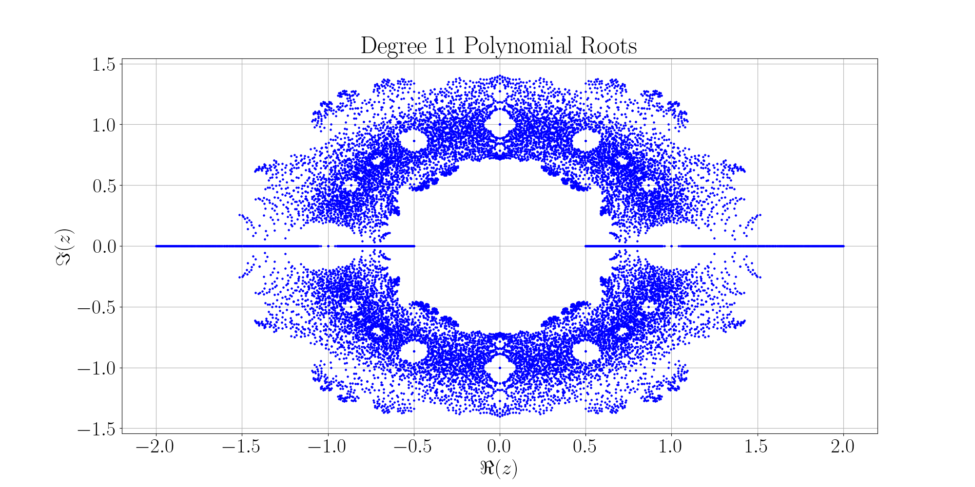
As an example, let's generate a plot of all the roots for all \(11^{th}\) degree polynomials with coefficients either +1 or -1. That is:
| \(a_0\) | \(a_1\) | \(a_2\) | \(a_3\) | \(a_4\) | \(a_5\) | \(a_6\) | \(a_7\) | \(a_8\) | \(a_9\) | \(a_{10}\) | \(a_{11}\) |
|---|---|---|---|---|---|---|---|---|---|---|---|
| -1 | -1 | -1 | -1 | -1 | -1 | -1 | -1 | -1 | -1 | -1 | -1 |
| -1 | -1 | -1 | -1 | -1 | -1 | -1 | -1 | -1 | -1 | -1 | 1 |
| -1 | -1 | -1 | -1 | -1 | -1 | -1 | -1 | -1 | -1 | 1 | -1 |
| -1 | -1 | -1 | -1 | -1 | -1 | -1 | -1 | -1 | -1 | 1 | 1 |
| -1 | -1 | -1 | -1 | -1 | -1 | -1 | -1 | -1 | 1 | -1 | -1 |
| -1 | -1 | -1 | -1 | -1 | -1 | -1 | -1 | -1 | 1 | -1 | 1 |
| -1 | -1 | -1 | -1 | -1 | -1 | -1 | -1 | -1 | 1 | 1 | -1 |
| -1 | -1 | -1 | -1 | -1 | -1 | -1 | -1 | -1 | 1 | 1 | 1 |
| \(\vdots\) | \(\vdots\) | \(\vdots\) | \(\vdots\) | \(\vdots\) | \(\vdots\) | \(\vdots\) | \(\vdots\) | \(\vdots\) | \(\vdots\) | \(\vdots\) | \(\vdots\) |
| 1 | 1 | 1 | 1 | 1 | 1 | 1 | 1 | 1 | 1 | 1 | 1 |
We'll use the polyroots method, which solves for the roots of a real polynomial equation by computing the eigenvalues of the companion matrix (using the LAPACK eigen solver DGEEV).
To get all the coefficient permutations, we will use a recursive algorithm, and pyplot-fortran to generate the plot.
Here is the code:
program main

use polyroots_module, only: polyroots, wp => polyroots_module_rk
use pyplot_module,    only: pyplot

implicit none

integer,parameter :: degree = 11 !! polynomial degree
integer,dimension(2) :: icoeffs = [-1,1] !! set of coefficients
integer,dimension(degree+1) :: a !! coefficients of polynomial
type(pyplot) :: plt  !! for making the plot
integer      :: ierr !! error code from [[polyroots]]
integer      :: j    !! counter

call plt%initialize(grid=.true.,xlabel='$\\Re(z)$',ylabel='$\\Im(z)$',&
                    title='Degree 11 Polynomial Roots',usetex=.true.,&
                    font_size=30, axes_labelsize=30, &
                    xtick_labelsize=30, ytick_labelsize=30, &
                    figsize=[20,10])
call generate(1)
call plt%showfig()

contains

    recursive subroutine generate(i)
    integer, intent(in) :: i
    integer :: ix
    real(wp),dimension(degree) :: zr, zi !! roots
    if (i > degree+1) then
        ! solve for this root and add it to the plot:
        call polyroots(degree,real(a,wp),zr,zi,ierr)
        call plt%add_plot(zr,zi,label='',linestyle='bo',markersize=2)
    else
        do ix = 1,size(icoeffs)
            a(i) = icoeffs(ix)
            call generate(i+1)
        end do
    end if
    end subroutine generate

end program main
The first set of roots, for \(a = [-1,-1,-1,-1,-1,-1,-1,-1,-1,-1,-1,-1]\), are: [\(-1\), \(\pm i\), \(\pm \sqrt3/2 \pm 0.5 i\), \(\pm 0.5 \pm \sqrt3/2\)].
The resultant plot with all the roots is shown here:
References
- A. Edelman and H. Murakami, "Polynomial roots from companion matrix eigenvalues", Math. Comp. 64 (1995), 763-776
- C. Moler, "ROOTS - Of Polynomials, That Is", MathWorks, 1991
- Abel–Ruffini theorem [wikipedia]
- Less verbose combinations, fortran-lang Discourse, Nov 2022