Jun 14, 2026
The FMIN function at Netlib is based on Richard Brent's classic localmin algorithm from [1].
The method uses a combination of golden section search and successive parabolic interpolation to compute the minimum of a 1D function without the necessity of evaluating any derivatives. There are Fortran 66 and ALGOL 60 versions of the method in the reference. I also have a modernized version here.
Let's show an example of how to use it for a simple orbital mechanics application.
Problem setup
Let's solve a trivial problem in orbital mechanics: computing the time of closest approach to a planet for a conic orbit. This is known as periapsis (or, for the Earth, perigee). We don't really need to use a minimizer to compute this, but it's a problem with a known solution that we can test the minimizer on.
We need various algorithms to do this:
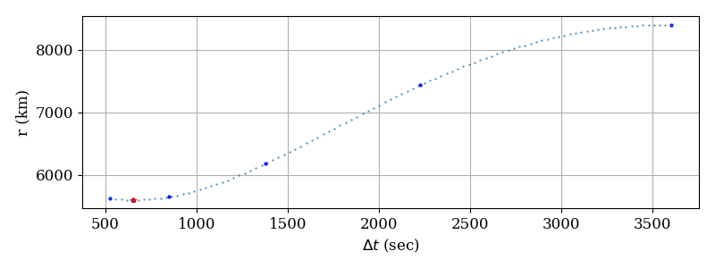
Given an initial elliptical orbit state, the Gooding routine pv3els will compute the time since last periapsis passage, so we have the "true" value to compare the results against. The function we pass to fmin to minimize will simply propagate the state (the independent variable is \(\Delta t\)) and return the radius magnitude (\(r\)). The point where the radius magnitude is minimized is the periapsis point we are looking for. The orbital period is used to set the upper time bound for the minimizer (we know there is only one periapsis passage per orbital period).
Example code
In our Fortran Package Manager manifest file, we define the two external dependencies we need:
[dependencies]
fmin = { git="https://github.com/jacobwilliams/fmin.git" }
fortran-astrodynamics-toolkit = { git="https://github.com/jacobwilliams/fortran-astrodynamics-toolkit.git" }
And the main program looks like this:
program main
  use fmin_module, wp => fmin_rk
  use fortran_astrodynamics_toolkit

  implicit none

  real(wp) :: p !! semiparameter [km]
  real(wp) :: period !! orbital period [sec]
  real(wp) :: dt !! time from initial state to periapsis [sec]
  real(wp),dimension(3) :: r, v !! position and velocity vectors [km] and [km/s]
  real(wp),dimension(6) :: rv0 !! initial state vector [km, km/s]
  real(wp),dimension(6) :: e0 !! Gooding orbital elements of the initial state
  integer :: n_evals = 0 !! number of function evaluations

  ! initial conditions (orbital elements):
  real(wp),parameter :: mu   = 398600.4418_wp  !! Earth grav. parameter [km^3/s^2]
  real(wp),parameter :: a    = 7000.0_wp       !! semi-major axis [km]
  real(wp),parameter :: ecc  = 0.2_wp          !! eccentricity
  real(wp),parameter :: inc  = 30.0_wp         !! inclination [deg]
  real(wp),parameter :: raan = 40.0_wp         !! right ascension of ascending node [deg]
  real(wp),parameter :: aop  = 60.0_wp         !! argument of perigee [deg]
  real(wp),parameter :: tru  = -45.0_wp        !! true anomaly [deg]
  real(wp),parameter :: tol  = 1.0e-6_wp       !! tolerance for fmin

  ! get the initial state vector and time from periapsis for the initial state:
  p = a * (1.0_wp - ecc**2)
  period = orbit_period(mu,a)
  call orbital_elements_to_rv(mu, p, ecc, inc, raan, aop, tru, r, v)
  rv0 = [r, v]
  call pv3els (mu, rv0, e0) ! e0(6) is the time from periapsis of the initial state

  ! call the minimizer:
  dt = fmin(func,0.0_wp,period,tol)

  ! print results
  write(*,'(A,F12.6,A)') 'DT to periapsis from fmin        = ', dt, ' sec'
  write(*,'(A,F12.6,A)') 'True initial time from periapsis = ', e0(6), ' sec'
  write(*,'(A,E12.3,A)') 'Error                            = ', dt + e0(6), ' sec'
  write(*,'(A,I0,A)')    'number of function evals         = ', n_evals, ' '

  contains

  function func(x) result(f)
    !! the function is to propagate from the initial state
    !! by the dt and compute the radius value
    real(wp),intent(in) :: x  !! indep. variable (dt)
    real(wp)            :: f  !! function value `f(x)` - radius magnitude
    real(wp),dimension(6) :: rvf
    call propagate(mu, rv0, x, rvf)
    f = norm2(rvf(1:3))
    n_evals = n_evals + 1
  end function func

end program main
Easy peasy!
Results
The result of running this program is:
DT to periapsis from fmin        =   652.983248 sec
True initial time from periapsis =  -652.983240 sec
Error                            =    0.875E-05 sec
number of function evals         = 12
So, it works! Using 12 function evaluations (i.e., kepler propagations of the orbit), the method has located the periapsis time to within about 8 \(\mu s\).
This sort of approach can also be used for less-trivial problems where we don't have a good analytical solution, and/or derivatives are unavailable or hard to obtain.
References
- R. Brent, "Algorithms for Minimization Without Derivatives", Prentice-Hall, 1973.
Jun 13, 2026

Reference [1] describes a numerical method for computing the derivative of a 1D function, using Neville's algorithm to extrapolate from a sequence of simple polynomial approximations based on interpolating points within specific bounds of a given point.
The original code in the published paper in 1980 was written in ALGOL 60. It seems as if a Fortran 77 translation was produced by David Kahaner at NIST circa 1989. I found the file on this NIST server where it has been sitting quietly since 1992 (originally this was an ftp server when I first found it). It's an interesting algorithm, and I included a modernized version in my NumDiff numerical differentiation library.
I also note that a version of the code is embedded within the Dataplot package.
But, there is a problem!
Here is a line of code in the original faccuracy function:
IF 16*ABS(H1)>ABS(H0) THEN H1:=SIGN(H1)*ABS(H0)/16;
Now, I know nothing about ALGOL 60, except that apparently John Backus (the creator of Fortran) was one of the committee members that developed it. Notice the SIGN function in this code.
This line was translated into Fortran 77 (where the function is renamed as FACCUR) as:
IF(16.*ABS(H1) .GT. ABS(H0)) H1 = SIGN(H1,1.)*ABS(H0)/16.
They are very similar, but note the SIGN function again.
In Fortran, the SIGN function (added in Fortran 77) is a little different since it has two arguments. While more flexible, it is a never-ending source of confusion, and I always have to look up the meaning of the two arguments. The following table summarizes the difference between the two:
| Language |
Syntax |
Description |
Reference |
| ALGOL 60 |
sign(E) |
the sign of the value of E (+1 for E>0, 0 for E=0, -1 for E<0) |
[2] |
| Fortran |
sign(A, B) |
the value of A with the sign of B |
[3] |
So, do you see the bug? SIGN(H1,1.) doesn't return the same thing that SIGN(H1) did in the original code. SIGN(H1,1.) returns the value of H1 with the sign of 1.0, which is always +H1, not the original intent at all! It really should have been translated to SIGN(1.0,H1), to give the +1/-1 of the original code. So, this bug is over 30 years old. Technically, the 0 case is still not handled the same, but that's a degenerate case that would never happen or give meaningful results in this context. But to be totally faithful we would need to use a function like this:
elemental real(wp) function sign_algol(x)
real(wp),intent(in) :: x
sign_algol = merge(0.0_wp, sign(1.0_wp,x), x==0.0_wp)
end function sign_algol
Other Languages
Python doesn't have a built-in sign function, but the numpy one behaves exactly like the ALGOL one. The advantage of the Fortran one is that it does support signed zeros, which the Numpy one does not appear to support (for that you need to use copysign). C++ also has a copysign function that does the same thing.
References
- J. Oliver, "Algorithm 017: An algorithm for numerical differentiation of a function of one real variable", Journal of Computational and Applied Mathematics 6 (2) (1980) 145-160. Fortran 77 code from NIST.
- J. W. Backus, F. L. Bauer, J. Green, C. Katz, J. McCarthy, A. J. Perlis, H. Rutishauser, K. Samelson, B. Vauquois, J. H. Wegstein, A. van Wijngaarden, M. Woodger Editor: P. Naur, "Revised Report on the Algorithmic Language ALGOL 60", Communications of the ACM, Volume 6, Issue 1
Pages 1 - 17, 01 January 1963.
- SIGN — Sign copying function [gcc.gnu.org]
- Numerical Differentiation, degenerateconic.com, Dec 04, 2016
May 30, 2026
Consider the problem of finding all the roots of a polynomial. This involves solving the following equation:
$$a_0 + a_1 x + a_2 x^2 + \cdots + a_n x^n = 0$$
This problem occurs in many different applications, such as computing atmospheric density in a spacecraft orbit simulation.
In general, both the coefficients and roots can be complex numbers. A special case involves only real coefficients. General methods exist for any degree polynomial, and custom methods also exist for polynomials of specific degree. The quadratic formula is the most famous analytical solution for polynomials of degree 2. In general, numerical methods are necessary to solve polynomials of degree 5 and higher.
Newton's method is frequently used, which requires an initial guess and an iterative procedure. Another elegant way to solve for all the roots at once is to find the eigenvalues of the companion matrix.
Fortran library

My polyroots-fortran library includes various methods to solve this problem. Many of the implementations have legacy going back decades (for example, from SLATEC). It's easy to incorporate into other codes using the Fortran Package Manager.
The available methods in the library are:
Example
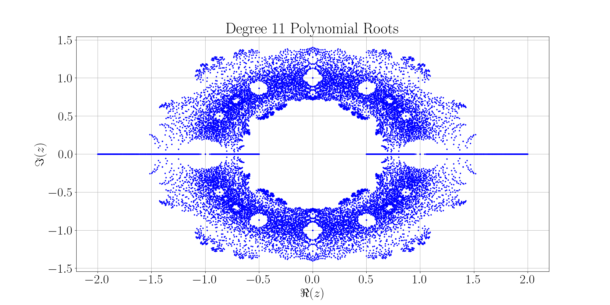
As an example, let's generate a plot of all the roots for all \(11^{th}\) degree polynomials with coefficients either +1 or -1. That is:
| \(a_0\) |
\(a_1\) |
\(a_2\) |
\(a_3\) |
\(a_4\) |
\(a_5\) |
\(a_6\) |
\(a_7\) |
\(a_8\) |
\(a_9\) |
\(a_{10}\) |
\(a_{11}\) |
| -1 |
-1 |
-1 |
-1 |
-1 |
-1 |
-1 |
-1 |
-1 |
-1 |
-1 |
-1 |
| -1 |
-1 |
-1 |
-1 |
-1 |
-1 |
-1 |
-1 |
-1 |
-1 |
-1 |
1 |
| -1 |
-1 |
-1 |
-1 |
-1 |
-1 |
-1 |
-1 |
-1 |
-1 |
1 |
-1 |
| -1 |
-1 |
-1 |
-1 |
-1 |
-1 |
-1 |
-1 |
-1 |
-1 |
1 |
1 |
| -1 |
-1 |
-1 |
-1 |
-1 |
-1 |
-1 |
-1 |
-1 |
1 |
-1 |
-1 |
| -1 |
-1 |
-1 |
-1 |
-1 |
-1 |
-1 |
-1 |
-1 |
1 |
-1 |
1 |
| -1 |
-1 |
-1 |
-1 |
-1 |
-1 |
-1 |
-1 |
-1 |
1 |
1 |
-1 |
| -1 |
-1 |
-1 |
-1 |
-1 |
-1 |
-1 |
-1 |
-1 |
1 |
1 |
1 |
| \(\vdots\) |
\(\vdots\) |
\(\vdots\) |
\(\vdots\) |
\(\vdots\) |
\(\vdots\) |
\(\vdots\) |
\(\vdots\) |
\(\vdots\) |
\(\vdots\) |
\(\vdots\) |
\(\vdots\) |
| 1 |
1 |
1 |
1 |
1 |
1 |
1 |
1 |
1 |
1 |
1 |
1 |
We'll use the polyroots method, which solves for the roots of a real polynomial equation by computing the eigenvalues of the companion matrix (using the LAPACK eigen solver DGEEV).
To get all the coefficient permutations, we will use a recursive algorithm, and pyplot-fortran to generate the plot.
Here is the code:
program main

use polyroots_module, only: polyroots, wp => polyroots_module_rk
use pyplot_module,    only: pyplot

implicit none

integer,parameter :: degree = 11 !! polynomial degree
integer,dimension(2) :: icoeffs = [-1,1] !! set of coefficients
integer,dimension(degree+1) :: a !! coefficients of polynomial
type(pyplot) :: plt  !! for making the plot
integer      :: ierr !! error code from [[polyroots]]
integer      :: j    !! counter

call plt%initialize(grid=.true.,xlabel='$\\Re(z)$',ylabel='$\\Im(z)$',&
                    title='Degree 11 Polynomial Roots',usetex=.true.,&
                    font_size=30, axes_labelsize=30, &
                    xtick_labelsize=30, ytick_labelsize=30, &
                    figsize=[20,10])
call generate(1)
call plt%showfig()

contains

    recursive subroutine generate(i)
    integer, intent(in) :: i
    integer :: ix
    real(wp),dimension(degree) :: zr, zi !! roots
    if (i > degree+1) then
        ! solve for this root and add it to the plot:
        call polyroots(degree,real(a,wp),zr,zi,ierr)
        call plt%add_plot(zr,zi,label='',linestyle='bo',markersize=2)
    else
        do ix = 1,size(icoeffs)
            a(i) = icoeffs(ix)
            call generate(i+1)
        end do
    end if
    end subroutine generate

end program main
The first set of roots, for \(a = [-1,-1,-1,-1,-1,-1,-1,-1,-1,-1,-1,-1]\), are: [\(-1\), \(\pm i\), \(\pm \sqrt3/2 \pm 0.5 i\), \(\pm 0.5 \pm \sqrt3/2\)].
The resultant plot with all the roots is shown here:
References
Jan 26, 2025

*From [A FORTRAN Coloring Book](https://archive.org/details/9780262610261) by Roger Kaufman (1978)*
Finding the \(x\) where a scalar function \(f(x) = 0\) is a common problem in numerical programming. There are numerous applications to this. In orbital mechanics, for example, we may want to find the time at which a spacecraft reaches a certain altitude, or enters the Earth's shadow. For these cases, the independent variable is time, and the function \(f\) requires integration of the equations of motion of the spacecraft (for example, by using an IVP solver such as DDEABM). Integrating to an event is often referred to as a "G-stop" feature in these types of applications.
One way to solve this problem is using a derivative-free bracketing method. For these, only function evaluations are used, and the algorithm begins within a set of bounds (\([x_a, x_b]\)) that bracket the root (i.e., \(sign~f(x_a) \ne sign~f(x_b)\)).
Over at the FORTRAN 77 Netlib graveyard, the classic zeroin root finding method can be found that implements such an algorithm, namely Brent's method by Australian mathematician Richard Brent from 1971.

In my roots-fortran library, I have modern Fortran implementations of this method and many others, as well as a lot of benchmark test cases. The library can be compiled for single (real32), double (real64), or quad (real128) precision reals.
For real64 numbers and convergence tolerance \(\epsilon\) = 1.0e-15, the following table lists the number of function evaluations for various methods to converge to the root for various test functions:
| \(f(x)\) |
\([x_a, x_b]\) |
\(x_{root}\) |
BS |
PE |
ITP |
TM |
BR |
AB |
MU |
CH |
| \((x - 1) e^{-x}\) |
\([0,1.5]\) |
1.0 |
46 |
10 |
11 |
9 |
11 |
10 |
9 |
9 |
| \(\cos x - x\) |
\([0,1.7]\) |
0.7390851332151607 |
47 |
8 |
9 |
8 |
8 |
8 |
7 |
8 |
| \(e^{x^2 + 7x - 30} - 1\) |
\([2.6,3.5]\) |
3.0 |
44 |
20 |
17 |
18 |
12 |
31 |
11 |
11 |
| \(x^3\) |
\([-0.5,1/3]\) |
0.0 |
17 |
50 |
16 |
46 |
40 |
38 |
61 |
17 |
| \(x^5\) |
\([-0.5,1/3]\) |
0.0 |
11 |
53 |
12 |
20 |
19 |
39 |
35 |
11 |
| \(\cos x - x^3\) |
\([0,4]\) |
0.8654740331016144 |
48 |
13 |
11 |
13 |
14 |
15 |
10 |
11 |
| \(x^3 - 1\) |
\([0.51,1.5]\) |
1.0 |
46 |
10 |
11 |
9 |
10 |
9 |
7 |
8 |
| \(x^2 ( x^2/3 + \sqrt{2} \sin x ) - \sqrt{3/18}\) |
\([0.1,1]\) |
0.3994222917109682 |
47 |
12 |
17 |
10 |
12 |
12 |
9 |
10 |
| \(x^3 + 1\) |
\([-1.8,0]\) |
-1.0 |
47 |
10 |
10 |
11 |
10 |
12 |
9 |
9 |
| \(\sin((x-7.14)^3)\) |
\([7,8]\) |
7.14 |
18 |
51 |
20 |
48 |
46 |
38 |
52 |
18 |
| \(e^{(x-3)^5} - 1\) |
\([2.6,3.6]\) |
3.0 |
11 |
55 |
12 |
24 |
26 |
41 |
29 |
11 |
| \(e^{(x-3)^5} - e^{x-1}\) |
\([4,5]\) |
4.267168304542125 |
44 |
53 |
45 |
11 |
14 |
58 |
20 |
14 |
| \(\pi - 1/x\) |
\([0.05,5]\) |
\(1 / \pi\) |
50 |
14 |
49 |
18 |
12 |
5 |
13 |
13 |
| \(4 - \tan x\) |
\([0,1.5]\) |
1.325817663668033 |
46 |
14 |
47 |
15 |
13 |
12 |
16 |
15 |
| \(2 x e^{-5} - 2 e^{-5x} + 1\) |
\([0,10]\) |
0.1382571550568241 |
52 |
13 |
16 |
13 |
13 |
11 |
13 |
13 |
The methods are: BS = Bisection, PE = Pegasus, ITP, TM = TOMS 748, BR = Brent, AB = Anderson Bjorck, MU = Muller, and CH = Chandrupatla.
There seems to be cottage industry of creating slight variations of this type of method. There are any number of recent papers on this topic, all claiming some improvement. In reality, a lot of the newer methods really aren't great. An obvious trick is a choose functions where your method behaves well. Another is to only compare against very simple methods (such as bisection or regula falsi, which are known to be inefficient). Finally, the most devious trick is to list the number of iterations of the method, rather than the number of function evaluations, which is basically a useless comparison that obscures the real cost for methods that have multiple function evaluations per iteration.
The Brent method is still one of the best performers. The Chandrupatla method from 1997 is also quite good. For the full set of test cases, see the roots-fortran git repo.
Minimization methods
A related type of algorithm are derivative-free minimization methods. The FMIN function at Netlib is based on Brent's original localmin algorithm (modern version here). The PRIMA library implements modern versions of M.J.D. Powell's derivative-free minimizers for multidimensional functions.
See also
- R. P. Brent, "An algorithm with guaranteed convergence for finding a zero of a function", The Computer Journal, Vol 14, No. 4., 1971.
- R. P. Brent, "Algorithms for Minimization Without Derivatives", Prentice-Hall, 1973.
- Gregory W. Chicares, Brent's method outperforms TOMS 748 [Let me illustrate...]
- T. R. Chandrupatla, "A new hybrid quadratic/bisection algorithm for
finding the zero of a nonlinear function without derivatives", Advances in
Engineering Software, Vol 28, 1997, pp. 145-149.
- M. J. D. Powell, "The BOBYQA algorithm for bound constrained optimization without derivatives," Department of Applied Mathematics and Theoretical Physics, Cambridge England, NA2009/06, 2009.
- polyroots-fortran -- Another modern Fortran library, specifically for finding the roots of polynomials.