Degenerate Conic

Brouwer-Lyddane Elements

The Brouwer-Lyddane elements are a set of "mean elements" used to describe the orbit of a spacecraft. Mean elements (as opposed to osculating elements) are used as a way to smooth out fluctuations of an orbit due to the zonal spherical harmonic terms. There are two flavors: short period (considering only J2) and long period (considering J2-J5). The equations were formulated in 1959 by Brouwer [1], and then improved in 1963 by Lyddane [2]. They have a long history of use in orbital mechanics.

Even though the earliest implementations of this method at NASA were in Fortran [3], I can't find any modern Fortran implementation of this algorithm. So, let's use our AI friend to create one! (see earlier post). Like last time, we will start with a C++ implementation from GMAT [4].

Input: reason, Output: pleasure

The result can be seen here. This conversion process was very smooth compared to the last time I tried something like this. Maybe the AI is getting better, or this is a more straightforward algorithm (or a little bit of both). It basically got it right the first time. I ended up having to massage it a little bit to get it into the form I wanted. It created a bunch of unit tests that also allowed for identifying a minor issue or two in the original code. Some changes from the original code are listed here:

• The Fortran version has selectable real kind values (so you can use single, double, or quad precision).
• It now accepts the planetary body terms as inputs, rather than having them be hard coded. So, it could potentially work for non-Earth applications.
• There was a bug in the original code if the inclination was greater than 175 deg.
• There was a potential divide by zero issue in the original code that I also fixed (if the orbit eccentricity was exactly zero).
• One interesting thing is that the AI decided to replace the error reporting mechanism in the original code (some kind of message reporting system in GMAT) with integer output codes from all the routines. Originally it implemented this in a slightly odd way (where stat was optional) but I just cleaned it up manually easily enough. Fortran does not yet have any kind of sane exception handling system, despite that being an oft-requested feature from users.
• The Fortran routines are snake_case rather than the original CamelCase. The AI just decided that was the way to go.

The main routines convert to/from Cartesian and the two flavors of mean elements:

• pure subroutine cartesian_to_brouwer_mean_short(mu, req, j2, cartesian, stat, blms)
• pure subroutine brouwer_mean_short_to_cartesian(mu, req, j2, blms, stat, cart)
• pure subroutine cartesian_to_brouwer_mean_long(mu, req, j2, j3, j4, j5, cartesian, stat, blml)
• pure subroutine brouwer_mean_long_to_cartesian(mu, req, j2, j3, j4, j5, blml, stat, cart)

The various unit tests perform singularity checks and round-trip type comparisons (where we start with a state in osculating orbital elements, then convert to Cartesian, then to mean elements, and then back to Cartesian, etc). These are all passing, which is a necessary but not really a sufficient condition for it all being correctly-implemented.

The code all seems to work pretty well. Is it all 100% correct? ¯\_(ツ)_/¯

Example

We can also perform a sanity check by propagating a state and visually comparing the osculating and mean elements. This test case can be found in the git repo here. Consider the following example LEO orbit state:

• Semimajor axis: 6800.0 km
• Eccentricity: 0.02 deg
• Inclination: 51.6 deg
• Right ascension of ascending node: 30 deg
• Argument of perigee: 40.0 deg
• True anomaly: 0.0 deg

Let's propagate this state at the Earth using the J2-J5 zonal harmonics. Inputs are:

• \(\mu\) = 398600.4415 (km\(^3\)/s\(^2\))
• \(r_{eq}\) = 6378.1363 (km)
• J2 = 1.082626925638815e-3
• J3 = -0.2532307818191774e-5
• J4 = -0.1620429990000000e-5
• J5 = -0.2270711043920343e-6

The equations of motion for this are given here:

subroutine gravity_j2_j3_j4_j5(r,mu,req,j2,j3,j4,j5,acc)

real(wp),dimension(3),intent(in)  :: r   !! satellite position vector [km]
real(wp),intent(in)               :: mu  !! central body gravitational parameter [km^3/s^2]
real(wp),intent(in)               :: req !! body equatorial radius [km]
real(wp),intent(in)               :: j2  !! j2 coefficient
real(wp),intent(in)               :: j3  !! j3 coefficient
real(wp),intent(in)               :: j4  !! j4 coefficient
real(wp),intent(in)               :: j5  !! j5 coefficient
real(wp),dimension(3),intent(out) :: acc !! gravity acceleration vector [km/s^2]

real(wp) :: rmag, r2, r3, z, z_r, z2_r2, z3_r3, z4_r4, &
            re_r, re_r2, re_r3, re_r4, re_r5, &
            f_r, f_z, mu_r3

r2 = dot_product(r, r)
rmag = sqrt(r2)
r3 = rmag * r2
z = r(3)
z_r = z / rmag
z2_r2 = z_r * z_r
z3_r3 = z2_r2 * z_r
z4_r4 = z2_r2 * z2_r2
re_r = req / rmag
re_r2 = re_r * re_r
re_r3 = re_r2 * re_r
re_r4 = re_r3 * re_r
re_r5 = re_r4 * re_r
mu_r3 = mu / r3

f_r = 1.0_wp + 1.5_wp * j2 * re_r2 * (1.0_wp - 5.0_wp * z2_r2) &
      + 2.5_wp * j3 * re_r3 * (3.0_wp * z_r - 7.0_wp * z3_r3) &
      - 0.625_wp * j4 * re_r4 * (3.0_wp - 42.0_wp * z2_r2 + 63.0_wp * z4_r4) &
      - 2.625_wp * j5 * re_r5 * (5.0_wp * z_r - 30.0_wp * z3_r3 + 33.0_wp * z4_r4 * z_r)

f_z = -3.0_wp * j2 * re_r2 * z_r &
      + 0.5_wp * j3 * re_r3 * (3.0_wp - 15.0_wp * z2_r2) &
      + 2.5_wp * j4 * re_r4 * (3.0_wp * z_r - 7.0_wp * z3_r3) &
      - 1.875_wp * j5 * re_r5 * (1.0_wp - 14.0_wp * z2_r2 + 21.0_wp * z4_r4)

acc = -mu_r3 * [r(1) * f_r, &
                r(2) * f_r, &
                (r(3) * f_r - rmag * f_z)]

end subroutine gravity_j2_j3_j4_j5

We can integrate this with any method we want, I'll use DDEABM (a variable step Adams method). Then, we use pyplot-fortran to make some plots.

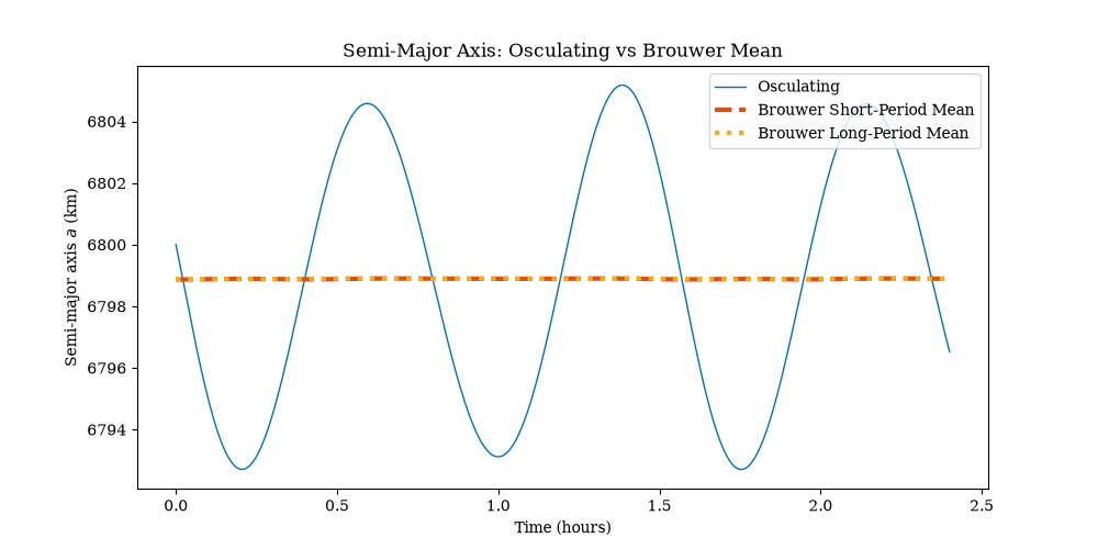
For the semimajor axis, we can clearly see how the mean element tracks the osculating one over time. In this case, there is not much difference between the short and long period mean:

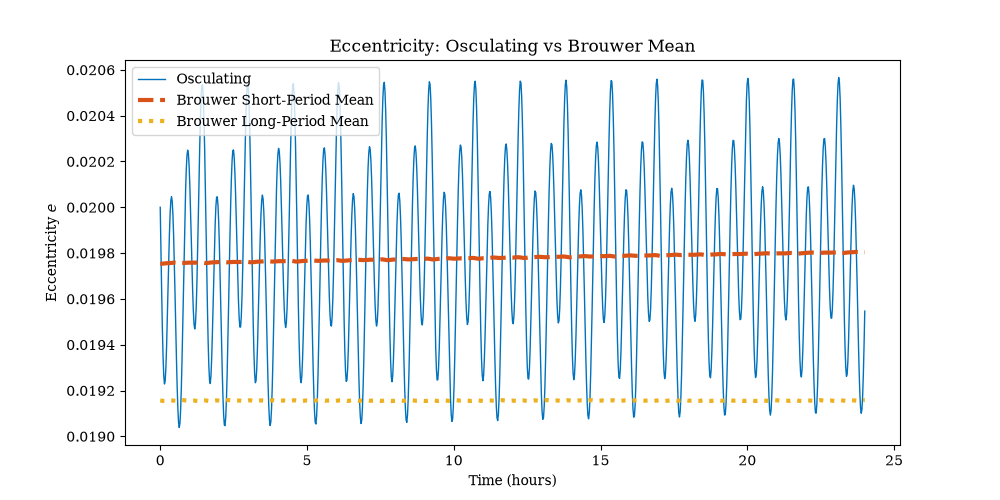
For eccentricity, it's a bit different. For a one-day propagation, the short-period mean tracks the eccentricity well, but the long-period one seems off:

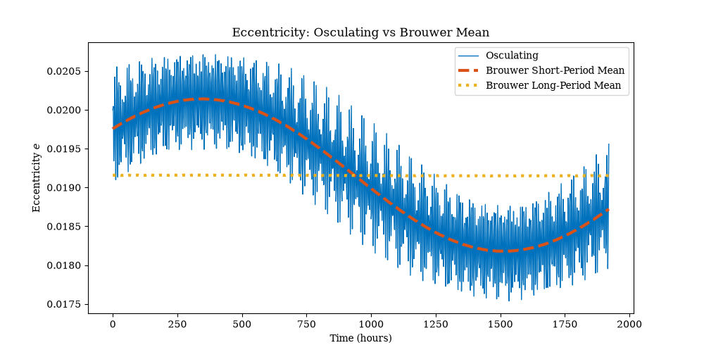
But if we propagate longer, we can see how the long-period terms come into play:

So, the results all look reasonable. To really validate this code, we'd need to (at a minimum) compare the outputs with the original code, but I haven't done that yet.

Summary

So, there you have it folks. Another somewhat-interesting AI-assisted conversion of an astrodynamics algorithm from C++ to Modern Fortran. The future is now, and we are all doomed!

Short biographies

Brouwer and Lyddane

Dirk Brower (1902-1966) was a Dutch-American astronomer/astrodynamicist, and professor at Yale University. He is the namesake of the Dirk Brouwer Award from the American Astronautical Society to honor significant technical contributions to space flight mechanics and astrodynamics. Russell H. Lyddane (1913-2001), a somewhat less well-known personage, was an American born in Washington DC. He worked at the Naval Weapons Laboratory in Dahlgren, Virginia from 1941-1964 (he served as Technical Director from 1956-1964).

References

1. Brouwer, D., "Solution of the Problem of Artificial Satellite Theory without Drag," Astronomical Journal, Vol. 64, Nov. 1959, pp. 378-397.
2. Lyddane, R. H., "Small Eccentricities or Inclinations in the Brouwer Theory of the Artificial Satellite," Astronomical Journal, Vol. 68, Oct. 1963, pp. 555-558.
3. E. A. Galbreath, "Brouwer-Lyddane Orbit Generator Routine", NASA GSFC, X-553-70-223, Sept. 1970. Note: there seems to be a version of this FORTRAN IV code given in an appendix of this NOAA document (Appendix F of the NOAA Polar Orbiter Data User's Guide, 1998-11-01).
4. NASA General Mission Analysis Tool (GMAT). [see the file: StateConversionUtil.cpp]
5. Brouwer-Lyddane Mean [FreeFlyer documentation].
6. J. Williams, Gooding Universal Elements, Oct 25, 2021 [degenerateconic.com]