Jun 14, 2026
The FMIN function at Netlib is based on Richard Brent's classic localmin algorithm from [1].
The method uses a combination of golden section search and successive parabolic interpolation to compute the minimum of a 1D function without the necessity of evaluating any derivatives. There are Fortran 66 and ALGOL 60 versions of the method in the reference. I also have a modernized version here.
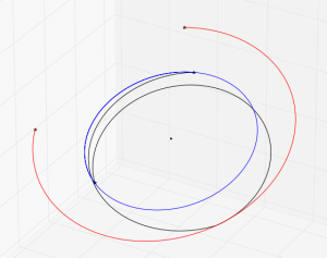
Let's show an example of how to use it for a simple orbital mechanics application.
Problem setup
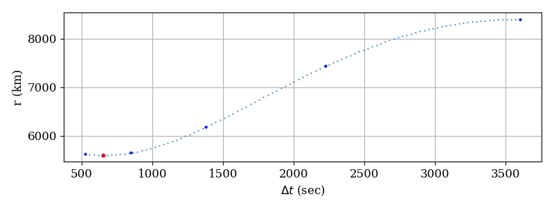
Let's solve a trivial problem in orbital mechanics: computing the time of closest approach to a planet for a conic orbit. This is known as periapsis (or, for the Earth, perigee). We don't really need to use a minimizer to compute this, but it's a problem with a known solution that we can test the minimizer on.
We need various algorithms to do this:
Given an initial elliptical orbit state, the Gooding routine pv3els will compute the time since last periapsis passage, so we have the "true" value to compare the results against. The function we pass to fmin to minimize will simply propagate the state (the independent variable is \(\Delta t\)) and return the radius magnitude (\(r\)). The point where the radius magnitude is minimized is the periapsis point we are looking for. The orbital period is used to set the upper time bound for the minimizer (we know there is only one periapsis passage per orbital period).
Example code
In our Fortran Package Manager manifest file, we define the two external dependencies we need:
[dependencies]
fmin = { git="https://github.com/jacobwilliams/fmin.git" }
fortran-astrodynamics-toolkit = { git="https://github.com/jacobwilliams/fortran-astrodynamics-toolkit.git" }
And the main program looks like this:
program main
  use fmin_module, wp => fmin_rk
  use fortran_astrodynamics_toolkit

  implicit none

  real(wp) :: p !! semiparameter [km]
  real(wp) :: period !! orbital period [sec]
  real(wp) :: dt !! time from initial state to periapsis [sec]
  real(wp),dimension(3) :: r, v !! position and velocity vectors [km] and [km/s]
  real(wp),dimension(6) :: rv0 !! initial state vector [km, km/s]
  real(wp),dimension(6) :: e0 !! Gooding orbital elements of the initial state
  integer :: n_evals = 0 !! number of function evaluations

  ! initial conditions (orbital elements):
  real(wp),parameter :: mu   = 398600.4418_wp  !! Earth grav. parameter [km^3/s^2]
  real(wp),parameter :: a    = 7000.0_wp       !! semi-major axis [km]
  real(wp),parameter :: ecc  = 0.2_wp          !! eccentricity
  real(wp),parameter :: inc  = 30.0_wp         !! inclination [deg]
  real(wp),parameter :: raan = 40.0_wp         !! right ascension of ascending node [deg]
  real(wp),parameter :: aop  = 60.0_wp         !! argument of perigee [deg]
  real(wp),parameter :: tru  = -45.0_wp        !! true anomaly [deg]
  real(wp),parameter :: tol  = 1.0e-6_wp       !! tolerance for fmin

  ! get the initial state vector and time from periapsis for the initial state:
  p = a * (1.0_wp - ecc**2)
  period = orbit_period(mu,a)
  call orbital_elements_to_rv(mu, p, ecc, inc, raan, aop, tru, r, v)
  rv0 = [r, v]
  call pv3els (mu, rv0, e0) ! e0(6) is the time from periapsis of the initial state

  ! call the minimizer:
  dt = fmin(func,0.0_wp,period,tol)

  ! print results
  write(*,'(A,F12.6,A)') 'DT to periapsis from fmin        = ', dt, ' sec'
  write(*,'(A,F12.6,A)') 'True initial time from periapsis = ', e0(6), ' sec'
  write(*,'(A,E12.3,A)') 'Error                            = ', dt + e0(6), ' sec'
  write(*,'(A,I0,A)')    'number of function evals         = ', n_evals, ' '

  contains

  function func(x) result(f)
    !! the function is to propagate from the initial state
    !! by the dt and compute the radius value
    real(wp),intent(in) :: x  !! indep. variable (dt)
    real(wp)            :: f  !! function value `f(x)` - radius magnitude
    real(wp),dimension(6) :: rvf
    call propagate(mu, rv0, x, rvf)
    f = norm2(rvf(1:3))
    n_evals = n_evals + 1
  end function func

end program main
Easy peasy!
Results
The result of running this program is:
DT to periapsis from fmin        =   652.983248 sec
True initial time from periapsis =  -652.983240 sec
Error                            =    0.875E-05 sec
number of function evals         = 12
So, it works! Using 12 function evaluations (i.e., kepler propagations of the orbit), the method has located the periapsis time to within about 8 \(\mu s\).
This sort of approach can also be used for less-trivial problems where we don't have a good analytical solution, and/or derivatives are unavailable or hard to obtain.
References
- R. Brent, "Algorithms for Minimization Without Derivatives", Prentice-Hall, 1973.
Nov 11, 2021
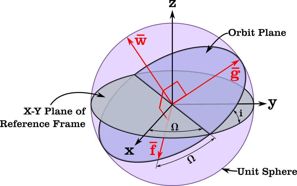
The Orbital Coordinate Frame used for Equinoctial Elements (see Reference [5])
Last time, I mentioned an alternative orbital element set different from the classical elements.
Modified equinoctial elements \((p,f,g,h,k,L)\) are another alternative that are applicable to all orbits and have nonsingular equations of motion (except for a singularity at \(i = \pi\)). They are defined as [1]:
- \(p = a (1 - e^2)\)
- \(f = e \cos (\omega + \Omega)\)
- \(g = e \sin (\omega + \Omega)\)
- \(h = \tan (i/2) \cos \Omega\)
- \(k = \tan (i/2) \sin \Omega\)
- \(L = \Omega + \omega + \nu\)
Where \(a\) is the semimajor axis, \(p\) is the semi-latus rectum, \(i\) is the inclination, \(e\) is the eccentricity, \(\omega\) is the argument of periapsis, \(\Omega\) is the right ascension of the ascending node, \(L\) is the true longitude, and \(\nu\) is the true anomaly. \((f,g)\) are the x and y components of the eccentricity vector in the orbital frame, and \((h,k)\) are the x and y components of the node vector in the orbital frame.
The conversion from Cartesian state (position and velocity) to modified equinoctial elements is given in this Fortran subroutine:
subroutine cartesian_to_equinoctial(mu,rv,evec)

use iso_fortran_env, only: wp => real64

implicit none

real(wp),intent(in)               :: mu    !! central body gravitational parameter (km^3/s^2)
real(wp),dimension(6),intent(in)  :: rv    !! Cartesian state vector
real(wp),dimension(6),intent(out) :: evec  !! Modified equinoctial element vector: [p,f,g,h,k,L]

real(wp),dimension(3) :: r,v,hvec,hhat,ecc,fhat,ghat,rhat,vhat
real(wp) :: hmag,rmag,p,f,g,h,k,L,kk,hh,s2,tkh,rdv

r = rv(1:3)
v = rv(4:6)

rdv      = dot_product(r,v)
rhat     = unit(r)
rmag     = norm2(r)
hvec     = cross(r,v)
hmag     = norm2(hvec)
hhat     = unit(hvec)
vhat     = (rmag*v - rdv*rhat)/hmag
p        = hmag*hmag / mu
k        = hhat(1)/(1.0_wp + hhat(3))
h        = -hhat(2)/(1.0_wp + hhat(3))
kk       = k*k
hh       = h*h
s2       = 1.0_wp+hh+kk
tkh      = 2.0_wp*k*h
ecc      = cross(v,hvec)/mu - rhat
fhat(1)  = 1.0_wp-kk+hh
fhat(2)  = tkh
fhat(3)  = -2.0_wp*k
ghat(1)  = tkh
ghat(2)  = 1.0_wp+kk-hh
ghat(3)  = 2.0_wp*h
fhat     = fhat/s2
ghat     = ghat/s2
f        = dot_product(ecc,fhat)
g        = dot_product(ecc,ghat)
L        = atan2(rhat(2)-vhat(1),rhat(1)+vhat(2))

evec = [p,f,g,h,k,L]

end subroutine cartesian_to_equinoctial
Where cross is a cross product function and unit is a unit vector function (\(\mathbf{u} = \mathbf{v} / |\mathbf{v}|\)).
The inverse routine (modified equinoctial to Cartesian) is:
subroutine equinoctial_to_cartesian(mu,evec,rv)

use iso_fortran_env, only: wp => real64

implicit none

real(wp),intent(in)               :: mu   !! central body gravitational parameter (km^3/s^2)
real(wp),dimension(6),intent(in)  :: evec !! Modified equinoctial element vector : [p,f,g,h,k,L]
real(wp),dimension(6),intent(out) :: rv   !! Cartesian state vector

real(wp) :: p,f,g,h,k,L,s2,r,w,cL,sL,smp,hh,kk,tkh
real(wp) :: x,y,xdot,ydot
real(wp),dimension(3) :: fhat,ghat

p = evec(1)
f = evec(2)
g = evec(3)
h = evec(4)
k = evec(5)
L = evec(6)

kk      = k*k
hh      = h*h
tkh     = 2.0_wp*k*h
s2      = 1.0_wp + hh + kk
cL      = cos(L)
sL      = sin(L)
w       = 1.0_wp + f*cL + g*sL
r       = p/w
smp     = sqrt(mu/p)
fhat(1) = 1.0_wp-kk+hh
fhat(2) = tkh
fhat(3) = -2.0_wp*k
ghat(1) = tkh
ghat(2) = 1.0_wp+kk-hh
ghat(3) = 2.0_wp*h
fhat    = fhat/s2
ghat    = ghat/s2
x       = r*cL
y       = r*sL
xdot    = -smp * (g + sL)
ydot    =  smp * (f + cL)

rv(1:3) = x*fhat + y*ghat
rv(4:6) = xdot*fhat + ydot*ghat

end subroutine equinoctial_to_cartesian
The equations of motion are:
subroutine modified_equinoctial_derivs(mu,evec,scn,evecd)

use iso_fortran_env, only: wp => real64

implicit none

real(wp),intent(in)               :: mu    !! central body gravitational parameter (km^3/s^2)
real(wp),dimension(6),intent(in)  :: evec  !! modified equinoctial element vector : [p,f,g,h,k,L]
real(wp),dimension(3),intent(in)  :: scn   !! Perturbation (in the RSW frame) (km/sec^2)
real(wp),dimension(6),intent(out) :: evecd !! derivative of `evec`

real(wp) :: p,f,g,h,k,L,c,s,n,sqrtpm,sl,cl,s2no2w,s2,w

p      = evec(1)
f      = evec(2)
g      = evec(3)
h      = evec(4)
k      = evec(5)
L      = evec(6)
s      = scn(1)
c      = scn(2)
n      = scn(3)
sqrtpm = sqrt(p/mu)
sl     = sin(L)
cl     = cos(L)
s2     = 1.0_wp + h*h + k*k
w      = 1.0_wp + f*cl + g*sl
s2no2w = s2*n / (2.0_wp*w)

evecd(1) = (2.0_wp*p*c/w) * sqrtpm
evecd(2) = sqrtpm * ( s*sl + ((w+1.0_wp)*cl+f)*c/w - g*n*(h*sl-k*cl)/w )
evecd(3) = sqrtpm * (-s*cl + ((w+1.0_wp)*sl+g)*c/w + f*n*(h*sl-k*cl)/w )
evecd(4) = sqrtpm * s2no2w * cl
evecd(5) = sqrtpm * s2no2w * sl
evecd(6) = sqrt(mu*p)*(w/p)**2 + sqrtpm * ((h*sl-k*cl)*n)/w

end subroutine modified_equinoctial_derivs
The 3-element scn vector contains the components of the perturbing acceleration (e.g. from a thrusting engine, other celestial bodies, etc.) in the directions perpendicular to the radius vector, in the "along track" direction, and the direction of the angular momentum vector.
Integration using modified equinoctial elements will generally be more efficient than a Cowell type integration of the Cartesian state elements. You only have to worry about the one singularity (note that there is also an alternate retrograde formulation where the singularity is moved to \(i = 0\)).
See also
References
- M. J. H. Walker, B. Ireland, Joyce Owens, "A Set of Modified Equinoctial Orbit Elements" Celestial Mechanics, Volume 36, Issue 4, p 409-419. (1985)
- Walker, M. J. H, "Erratum - a Set of Modified Equinoctial Orbit Elements" Celestial Mechanics, Volume 38, Issue 4, p 391-392. (1986)
- Broucke, R. A. & Cefola, P. J., "On the Equinoctial Orbit Elements" Celestial Mechanics, Volume 5, Issue 3, p 303-310. (1972)
- D. A. Danielson, C. P. Sagovac, B. Neta, L. W. Early, "Semianalytic Satellite Theory", Naval Postgraduate School Department of Mathematics, 1995
- P. J. Cefola, "Equinoctial orbit elements - Application to artificial satellite orbits", Astrodynamics Conference, 11-12 September 1972.
Oct 25, 2021
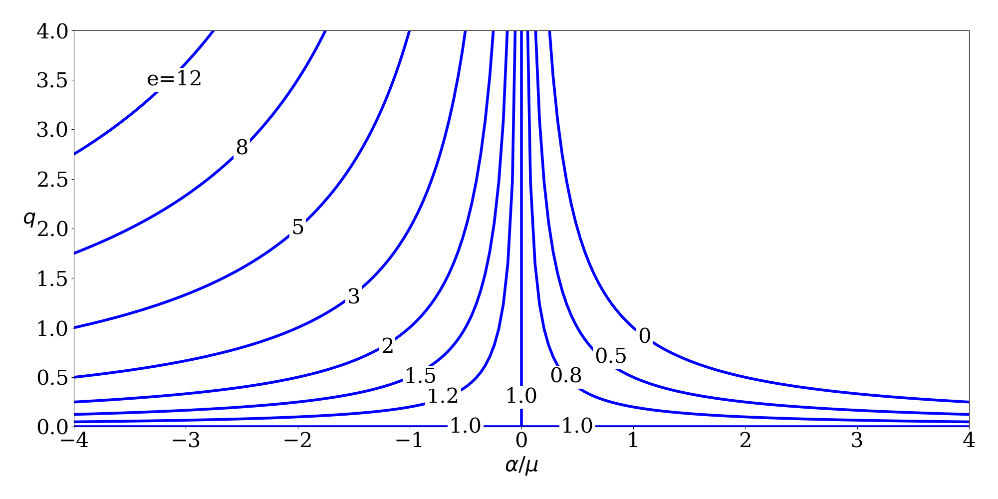
Variation of $q$ with $\alpha/\mu ~(=1/a)$ for selected values of $e$. (see Reference [1])
There are various different 6-element sets that can be used to represent the state (position and velocity) of a spacecraft. The classical Keplerian element set (\(a\), \(e\), \(i\), \(\Omega\), \(\omega\), \(\nu\)) is perhaps the most common, but not the only one. The Gooding universal element set [1] is:
- \(\alpha\) : twice the negative energy per unit mass (\(2 \mu / r - v^2\) or \(\mu/a\))
- \(q\) : periapsis radius magnitude (a.k.a. \(r_p\))
- \(i\) : inclination
- \(\Omega\) : right ascension of the ascending node
- \(\omega\) : argument of periapsis
- \(\tau\) : time since last periapsis passage
The nice thing about this set is that it is always defined, even for parabolas and rectilinear orbits (which other orbital element sets tend to ignore). A table from [1] shows the relationship between \(\alpha\) and \(q\) for the different types of conics:
|
\(\alpha > 0\) |
\(\alpha = 0\) |
\(\alpha < 0\) |
| \(q > 0\) |
general ellipse |
general parabola |
general hyperbola |
| \(q = 0\) |
rectilinear ellipse |
rectilinear parabola |
rectilinear hyperbola |
One advantage of this formulation is for trajectory optimization purposes, since if \(\alpha\) is an optimization variable, the orbit can transition from an ellipse to a hyperbola while iterating without encountering any singularities (which is not true if semimajor axis and eccentricity are being used, since \(a \rightarrow \infty\) for a parabola and then becomes negative for a hyperbola).
Gooding's original paper from 1988 includes Fortran 77 code for the transformations to and from position and velocity, coded with great care to avoid loss of accuracy due to numerical issues. Two other papers [2-3] also include some components of the algorithm. Modernized versions of these routines can be found in the Fortran Astrodynamics Toolkit. For example, a modernized version of ekepl1 (from [2]) for solving Kepler's equation:
pure function ekepl1(em, e)
  !!  Solve kepler's equation, `em = ekepl - e*sin(ekepl)`,
  !!  with legendre-based starter and halley iterator

  implicit none

  real(wp) :: ekepl1
  real(wp),intent(in) :: em
  real(wp),intent(in) :: e

  real(wp) :: c,s,psi,xi,eta,fd,fdd,f

  real(wp),parameter :: testsq = 1.0e-8_wp

  c = e*cos(em)
  s = e*sin(em)
  psi = s/sqrt(1.0_wp - c - c + e*e)

  do
    xi = cos(psi)
    eta = sin(psi)
    fd = (1.0_wp - c*xi) + s*eta
    fdd = c*eta + s*xi
    f = psi - fdd
    psi = psi - f*fd/(fd*fd - 0.5_wp*f*fdd)
    if (f*f < testsq) exit
   end do

   ekepl1 = em + psi

end function ekepl1
The Gooding universal element set can be found in NASA's Copernicus tool, and is being used in the design and optimization of the Artemis I trajectory.
See also
References
- R. H. Gooding, "On universal elements, and conversion procedures to and from position and velocity" Celestial Mechanics 44 (1988), 283-298.
- A. W. Odell, R. H. Gooding, "Procedures for solving Kepler's equation" Celestial Mechanics 38 (1986), 307-334.
- R. H. Gooding, A. W. Odell. "The hyperbolic Kepler equation (and the elliptic equation revisited)" Celestial Mechanics 44 (1988), 267-282.
- J, Williams, J. S. Senent, and D. E. Lee, "Recent improvements to the copernicus trajectory design and optimization system", Advances in the Astronautical Sciences 143, January 2012 (AAS 12-236)
- G. Hintz, "Survey of Orbit Element Sets", Journal of Guidance Control and Dynamics, 31(3):785-790, May 2008
Dec 10, 2018
I came across this old NASA document from 1963, where a cross product subroutine is defined in Fortran (based on some of the other routines given, it looks like they were using FORTRAN II):
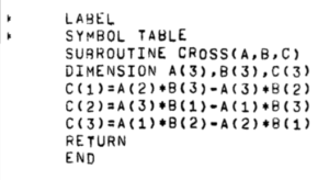
A cross product function is always a necessary procedure in any orbital mechanics simulation (for example when computing the angular momentum vector \(\mathbf{h} = \mathbf{r} \times \mathbf{v}\)). The interesting thing is that this subroutine will still compile today with any Fortran compiler. Of course, there are a few features used here that are deemed obsolescent in modern Fortran (fixed-form source, implicit typing, and the DIMENSION statement). Also it is using single precision reals (which no one uses anymore in this field). A modernized version would look something like this:
subroutine cross(a,b,c)
implicit none
real(wp),dimension(3),intent(in) :: a,b
real(wp),dimension(3),intent(out) :: c
c(1) = a(2)*b(3)-a(3)*b(2)
c(2) = a(3)*b(1)-a(1)*b(3)
c(3) = a(1)*b(2)-a(2)*b(1)
end subroutine cross
But, basically, except for declaring the real kind, it does exactly the same thing as the one from 1963. The modern routine would presumably be put in a module (in which the WP kind parameter is accessible), for example, a vector utilities module. While a subroutine is perfectly acceptable for this case, my preference would be to use a function like so:
pure function cross(a,b) result(c)
implicit none
real(wp),dimension(3),intent(in) :: a,b
real(wp),dimension(3) :: c
c(1) = a(2)*b(3)-a(3)*b(2)
c(2) = a(3)*b(1)-a(1)*b(3)
c(3) = a(1)*b(2)-a(2)*b(1)
end function cross
This one is a function that return a \(\mathrm{3} \times \mathrm{1}\) vector, and is explicitly declared to be PURE (which can allow for more aggressive code optimizations from the compiler).
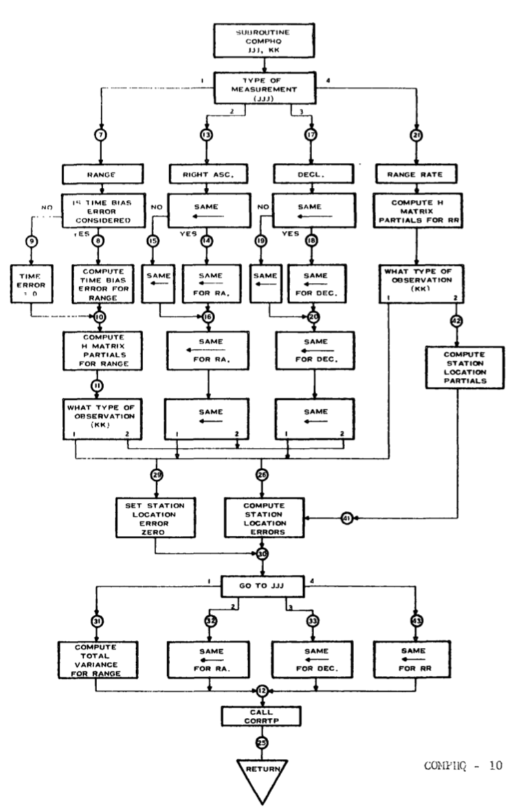
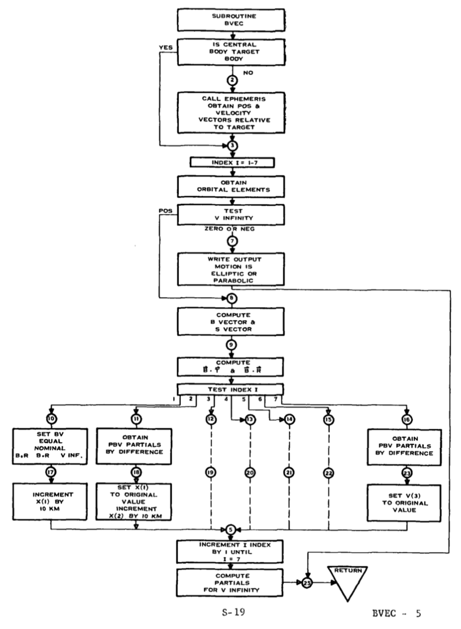
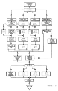
This document, which is the programmer's manual for an interplanetary error propagation program, contains a lot of other Fortran gems. It also has some awesome old school flow charts:

See also
Apr 04, 2018
Many of NASA's workhorse spacecraft trajectory optimization tools are written in Fortran or have Fortran components (e.g., OTIS, MALTO, Mystic, and Copernicus). None of it is really publicly-available however. There are some freely-available Fortran codes around for general-purpose orbital mechanics applications. Including:
You can also find some old Fortran gems in various papers on the NASA Technical Reports Server.
See also
- J. Williams, R. D. Falck, and I. B. Beekman. "Application of Modern Fortran to Spacecraft Trajectory Design and Optimization", 2018 Space Flight Mechanics Meeting, AIAA SciTech Forum, (AIAA 2018-1451)
Mar 14, 2015
*Earth-Mars Free Return*
Let's try using the Fortran Astrodynamics Toolkit and Pikaia to solve a real-world orbital mechanics problem. In this case, computing the optimal Earth-Mars free return trajectory in the year 2018. This is a trajectory that departs Earth, and then with no subsequent maneuvers, flies by Mars and returns to Earth. The building blocks we need to do this are:
- An ephemeris of the Earth and Mars [DE405]
- A Lambert solver [1]
- Some equations for hyperbolic orbits [given below]
- An optimizer [Pikaia]
The \(\mathbf{v}_{\infty}\) vector of a hyperbolic planetary flyby (using patched conic assumptions) is simply the difference between the spacecraft's heliocentric velocity and the planet's velocity:
- \(\mathbf{v}_{\infty} = \mathbf{v}_{heliocentric} - \mathbf{v}_{planet}\)
The hyperbolic turning angle \(\Delta\) is the angle between \(\mathbf{v}_{\infty}^{-}\) (the \(\mathbf{v}_{\infty}\) before the flyby) and the \(\mathbf{v}_{\infty}^{+}\) (the \(\mathbf{v}_{\infty}\) vector after the flyby). The turning angle can be used to compute the flyby periapsis radius \(r_p\) using the equations:
- \(e = \frac{1}{\sin(\Delta/2)}\)
- \(r_p = \frac{\mu}{v_{\infty}^2}(e-1)\)
So, from the Lambert solver, we can obtain Earth to Mars, and Mars to Earth trajectories (and the heliocentric velocities at each end). These are used to compute the \(\mathbf{v}_{\infty}\) vectors at: Earth departure, Mars flyby (both incoming and outgoing vectors), and Earth return.
There are three optimization variables:
- The epoch of Earth departure [modified Julian date]
- The outbound flight time from Earth to Mars [days]
- The return flyby time from Mars to Earth [days]
There are also two constraints on the heliocentric velocity vectors before and after the flyby at Mars:
- The Mars flyby must be unpowered (i.e., no propulsive maneuver is performed). This means that the magnitude of the incoming (\(\mathbf{v}_{\infty}^-\)) and outgoing (\(\mathbf{v}_{\infty}^+\)) vectors must be equal.
- The periapsis flyby radius (\(r_p\)) must be greater than some minimum value (say, 160 km above the Martian surface).
For the objective function (the quantity that is being minimized), we will use the sum of the Earth departure and return \(\mathbf{v}_{\infty}\) vector magnitudes. To solve this problem using Pikaia, we need to create a fitness function, which is given below:
subroutine obj_func(me,x,f)

!Pikaia fitness function for an Earth-Mars free return

use fortran_astrodynamics_toolkit

implicit none

class(pikaia_class),intent(inout) :: me !pikaia class
real(wp),dimension(:),intent(in) :: x !optimization variable vector
real(wp),intent(out) :: f !fitness value

real(wp),dimension(6) :: rv_earth_0, rv_mars, rv_earth_f
real(wp),dimension(3) :: v1,v2,v3,v4,vinf_0,vinf_f,vinfm,vinfp
real(wp) :: jd_earth_0,jd_mars,jd_earth_f,&
dt_earth_out,dt_earth_return,&
rp_penalty,vinf_penalty,e,delta,rp,vinfmag

real(wp),parameter :: mu_sun = 132712440018.0_wp !sun grav param [km3/s2]
real(wp),parameter :: mu_mars = 42828.0_wp !mars grav param [km3/s2]
real(wp),parameter :: rp_mars_min = 3390.0_wp+160.0_wp !min flyby radius at mars [km]
real(wp),parameter :: vinf_weight = 1000.0_wp !weights for the
real(wp),parameter :: rp_weight = 10.0_wp ! penalty functions

!get times:
jd_earth_0 = mjd_to_jd(x(1)) !julian date of earth departure
dt_earth_out = x(2) !outbound flyby time [days]
dt_earth_return = x(3) !return flyby time [days]
jd_mars = jd_earth_0 + dt_earth_out !julian date of mars flyby
jd_earth_f = jd_mars + dt_earth_return !julian date of earth arrival

!get earth/mars locations (wrt Sun):
call get_state(jd_earth_0,3,11,rv_earth_0) !earth at departure
call get_state(jd_mars, 4,11,rv_mars) !mars at flyby
call get_state(jd_earth_f,3,11,rv_earth_f) !earth at arrival

!compute lambert maneuvers:
call lambert(rv_earth_0,rv_mars, dt_earth_out*day2sec, mu_sun,v1,v2) !outbound
call lambert(rv_mars, rv_earth_f,dt_earth_return*day2sec,mu_sun,v3,v4) !return

!compute v-inf vectors:
vinf_0 = v1 - rv_earth_0(4:6) !earth departure
vinfm = v2 - rv_mars(4:6) !mars flyby (incoming)
vinfp = v3 - rv_mars(4:6) !mars flyby (outgoing)
vinf_f = v4 - rv_earth_f(4:6) !earth return

!the turning angle is the angle between vinf- and vinf+
delta = angle_between_vectors(vinfm,vinfp) !turning angle [rad]
vinfmag = norm2(vinfm) !vinf vector mag (incoming) [km/s]
e = one/sin(delta/two) !eccentricity
rp = mu_mars/(vinfmag*vinfmag)*(e-one) !periapsis radius [km]

!the constraints are added to the fitness function as penalties:
if (rp>=rp_mars_min) then
    rp_penalty = zero !not active
else
    rp_penalty = rp_mars_min - rp
end if
vinf_penalty = abs(norm2(vinfm) - norm2(vinfp))

!fitness function (to maximize):
f = - ( norm2(vinf_0) + &
    norm2(vinf_f) + &
    vinf_weight*vinf_penalty + &
    rp_weight*rp_penalty )

end subroutine obj_func
The lambert routine called here is simply a wrapper to solve_lambert_gooding that computes both the "short way" and "long way" transfers, and returns the one with the lowest total \(\Delta v\). The two constraints are added to the objective function as penalties (to be driven to zero). Pikaia is then initialized and called by:
program flyby

use pikaia_module
use fortran_astrodynamics_toolkit

implicit none

integer,parameter :: n = 3

type(pikaia_class) :: p
real(wp),dimension(n) :: x,xl,xu
integer :: status,iseed
real(wp) :: f

!set random number seed:
iseed = 371

!bounds:
xl = [jd_to_mjd(julian_date(2018,1,1,0,0,0)), 100.0_wp,100.0_wp]
xu = [jd_to_mjd(julian_date(2018,12,31,0,0,0)),400.0_wp,400.0_wp]

call p%init(n,xl,xu,obj_func,status,&
            ngen = 1000, &
            np = 200, &
            nd = 9, &
            ivrb = 0, &
            convergence_tol = 1.0e-6_wp, &
            convergence_window = 200, &
            initial_guess_frac = 0.0_wp, &
            iseed = iseed )

call p%solve(x,f,status)

end program flyby
The three optimization variables are bounded: the Earth departure epoch must occur sometime in 2018, and the outbound and return flight times must each be between 100 and 400 days.
Running this program, we can get different solutions (depending on the value set for the random seed, and also the Pikaia settings). The best one I've managed to get with minimal tweaking is this:
- Earth departure epoch: MJD 58120 (Jan 2, 2018)
- Outbound flight time: 229 days
- Return flight time: 271 days
Which is similar to the solution shown in [2].
References
- R.H. Gooding, "A procedure for the solution of Lambert's orbital boundary-value problem", Celestial Mechanics and Dynamical Astronomy, Vol. 48, No. 2, 1990.
- Dennis Tito's 2021 Human Mars Flyby Mission Explained. SPACE.com, February 27, 2014.
- J.E. Prussing, B.A. Conway, "Orbital Mechanics", Oxford University Press, 1993.
Feb 08, 2015

The IAU Working Group on Cartographic Coordinates and Rotational Elements (WGCCRE) is the keeper of official models that describe the cartographic coordinates and rotational elements of planetary bodies (such as the Earth, satellites, minor planets, and comets). Periodically, they release a report containing the coefficients to compute body orientations, based on the latest data available. These coefficients allow one to compute the rotation matrix from the ICRF frame to a body-fixed frame (for example, IAU Earth) by giving the direction of the pole vector and the prime meridian location as functions of time. An example Fortran module illustrating this for the IAU Earth frame is given below. The coefficients are taken from the 2009 IAU report [Reference 1]. Note that the IAU models are also available in SPICE (as "IAU_EARTH", "IAU_MOON", etc.). For Earth, the IAU model is not suitable for use in applications that require the highest possible accuracy (for that a more complex model would be necessary), but is quite acceptable for many applications.
module iau_orientation_module

use, intrinsic :: iso_fortran_env, only: wp => real64

implicit none

private

!constants:
real(wp),parameter :: zero = 0.0_wp
real(wp),parameter :: one = 1.0_wp
real(wp),parameter :: pi = acos(-one)
real(wp),parameter :: pi2 = pi/2.0_wp
real(wp),parameter :: deg2rad = pi/180.0_wp
real(wp),parameter :: sec2day = one/86400.0_wp
real(wp),parameter :: sec2century = one/3155760000.0_wp

public :: icrf_to_iau_earth

contains

!Rotation matrix from ICRF to IAU_EARTH
pure function icrf_to_iau_earth(et) result(rotmat)

implicit none

real(wp),intent(in) :: et !ephemeris time [sec from J2000]
real(wp),dimension(3,3) :: rotmat !rotation matrix

real(wp) :: w,dec,ra,d,t
real(wp),dimension(3,3) :: tmp

d = et * sec2day !days from J2000
t = et * sec2century !Julian centuries from J2000

ra = ( - 0.641_wp * t ) * deg2rad
dec = ( 90.0_wp - 0.557_wp * t ) * deg2rad
w = ( 190.147_wp + 360.9856235_wp * d ) * deg2rad

!it is a 3-1-3 rotation:
tmp = matmul( rotmat_x(pi2-dec), rotmat_z(pi2+ra) )
rotmat = matmul( rotmat_z(w), tmp )

end function icrf_to_iau_earth

!The 3x3 rotation matrix for a rotation about the x-axis.
pure function rotmat_x(angle) result(rotmat)

implicit none

real(wp),dimension(3,3) :: rotmat !rotation matrix
real(wp),intent(in) :: angle !angle [rad]

real(wp) :: c,s

c = cos(angle)
s = sin(angle)

rotmat = reshape([one, zero, zero, &
                  zero, c, -s, &
                  zero, s, c],[3,3])

end function rotmat_x

!The 3x3 rotation matrix for a rotation about the z-axis.
pure function rotmat_z(angle) result(rotmat)

implicit none

real(wp),dimension(3,3) :: rotmat !rotation matrix
real(wp),intent(in) :: angle !angle [rad]

real(wp) :: c,s

c = cos(angle)
s = sin(angle)

rotmat = reshape([ c, -s, zero, &
                   s, c, zero, &
                   zero, zero, one ],[3,3])

end function rotmat_z

end module iau_orientation_module
References
- B. A. Archinal, et al., "Report of the IAU Working Group on Cartographic Coordinates and Rotational Elements: 2009", Celest Mech Dyn Astr (2011) 109:101-135.
- J. Williams, Fortran Astrodynamics Toolkit - iau_orientation_module [GitHub]
Jan 29, 2015

The Standards of Fundamental Astronomy (SOFA) library is a very nice collection of routines that implement various IAU algorithms for fundamental astronomy computations. Versions are available in Fortran and C. Unfortunately, the Fortran version is written to be of maximum use to astronomers who frequently travel back in time to 1977 and compile the code on their UNIVAC (i.e., it is fixed-format Fortran 77). To assist 21st century users, I uploaded a little Python script called SofaMerge to Github. This script can make your life easier by merging all the individual source files into a single Fortran module file (with a few cosmetic updates along the way). It doesn't yet include any fixed to free format changes, but that could be easily added later.
Jan 26, 2015
The gravitational potential of a non-homogeneous celestial body at radius \(r\), latitude \(\phi\) , and longitude \(\lambda\) can be represented in spherical coordinates as:
$$
U = \frac{\mu}{r} [ 1 + \sum\limits_{n=2}^{n_{max}} \sum\limits_{m=0}^{n} \left( \frac{r_e}{r} \right)^n P_{n,m}(\sin \phi) ( C_{n,m} \cos m\lambda + S_{n,m} \sin m\lambda ) ]
$$
Where \(r_e\) is the radius of the body, \(\mu\) is the gravitational parameter of the body, \(C_{n,m}\) and \(S_{n,m}\) are spherical harmonic coefficients, \(P_{n,m}\) are Associated Legendre Functions, and \(n_{max}\) is the desired degree and order of the approximation. The acceleration of a spacecraft at this location is the gradient of this potential. However, if the conventional representation of the potential given above is used, it will result in singularities at the poles \((\phi = \pm 90^{\circ})\), since the longitude becomes undefined at these points. (Also, evaluation on a computer would be relatively slow due to the number of sine and cosine terms).
A geopotential formulation that eliminates the polar singularity was devised by Samuel Pines in the early 1970s [1]. Over the years, various implementations and refinements of this algorithm and other similar algorithms have been published [2-7], mostly at the Johnson Space Center. The Fortran 77 code in Mueller [2] and Lear [4-5] is easily translated into modern Fortran. The Pines algorithm code from Spencer [3] appears to contain a few bugs, so translation is more of a challenge. A modern Fortran version (with bugs fixed) is presented below:
subroutine gravpot(r,nmax,re,mu,c,s,acc)

use, intrinsic :: iso_fortran_env, only: wp => real64

implicit none

real(wp),dimension(3),intent(in) :: r !position vector
integer,intent(in) :: nmax !degree/order
real(wp),intent(in) :: re !body radius
real(wp),intent(in) :: mu !grav constant
real(wp),dimension(nmax,0:nmax),intent(in) :: c !coefficients
real(wp),dimension(nmax,0:nmax),intent(in) :: s !
real(wp),dimension(3),intent(out) :: acc !grav acceleration

!local variables:
real(wp),dimension(nmax+1) :: creal, cimag, rho
real(wp),dimension(nmax+1,nmax+1) :: a,d,e,f
integer :: nax0,i,j,k,l,n,m
real(wp) :: rinv,ess,t,u,r0,rhozero,a1,a2,a3,a4,fac1,fac2,fac3,fac4
real(wp) :: ci1,si1

real(wp),parameter :: zero = 0.0_wp
real(wp),parameter :: one = 1.0_wp

!JW : not done in original paper,
!     but seems to be necessary
!     (probably assumed the compiler
!      did it automatically)
a = zero
d = zero
e = zero
f = zero

!get the direction cosines ess, t and u:

nax0 = nmax + 1
rinv = one/norm2(r)
ess  = r(1) * rinv
t    = r(2) * rinv
u    = r(3) * rinv

!generate the functions creal, cimag, a, d, e, f and rho:

r0       = re*rinv
rhozero  = mu*rinv    !JW: typo in original paper
rho(1)   = r0*rhozero
creal(1) = ess
cimag(1) = t
d(1,1)   = zero
e(1,1)   = zero
f(1,1)   = zero
a(1,1)   = one

do i=2,nax0

    if (i/=nax0) then !JW : to prevent access
        ci1 = c(i,1)  !     to c,s outside bounds
        si1 = s(i,1)
    else
        ci1 = zero
        si1 = zero
    end if

    rho(i)   = r0*rho(i-1)
    creal(i) = ess*creal(i-1) - t*cimag(i-1)
    cimag(i) = ess*cimag(i-1) + t*creal(i-1)
    d(i,1)   = ess*ci1 + t*si1
    e(i,1)   = ci1
    f(i,1)   = si1
    a(i,i)   = (2*i-1)*a(i-1,i-1)
    a(i,i-1) = u*a(i,i)

    do k=2,i

        if (i/=nax0) then
            d(i,k) = c(i,k)*creal(k)   + s(i,k)*cimag(k)
            e(i,k) = c(i,k)*creal(k-1) + s(i,k)*cimag(k-1)
            f(i,k) = s(i,k)*creal(k-1) - c(i,k)*cimag(k-1)
        end if

        !JW : typo here in original paper
        ! (should be GOTO 1, not GOTO 10)
        if (i/=2) then
            L = i-2
            do j=1,L
                a(i,i-j-1) = (u*a(i,i-j)-a(i-1,i-j))/(j+1)
            end do
        end if

    end do

end do

!compute auxiliary quantities a1, a2, a3, a4

a1 = zero
a2 = zero
a3 = zero
a4 = rhozero*rinv

do n=2,nmax

    fac1 = zero
    fac2 = zero
    fac3 = a(n,1)  *c(n,0)
    fac4 = a(n+1,1)*c(n,0)

    do m=1,n
        fac1 = fac1 + m*a(n,m)    *e(n,m)
        fac2 = fac2 + m*a(n,m)    *f(n,m)
        fac3 = fac3 +   a(n,m+1)  *d(n,m)
        fac4 = fac4 +   a(n+1,m+1)*d(n,m)
    end do

    a1 = a1 + rinv*rho(n)*fac1
    a2 = a2 + rinv*rho(n)*fac2
    a3 = a3 + rinv*rho(n)*fac3
    a4 = a4 + rinv*rho(n)*fac4

end do

!gravitational acceleration vector:

acc(1) = a1 - ess*a4
acc(2) = a2 - t*a4
acc(3) = a3 - u*a4

end subroutine gravpot
References
- S. Pines. "Uniform Representation of the Gravitational Potential and its Derivatives", AIAA Journal, Vol. 11, No. 11, (1973), pp. 1508-1511.
- A. C. Mueller, "A Fast Recursive Algorithm for Calculating the Forces due to the Geopotential (Program: GEOPOT)", JSC Internal Note 75-FM-42, June 9, 1975.
- J. L. Spencer, "Pines Nonsingular Gravitational Potential Derivation, Description and Implementation", NASA Contractor Report 147478, February 9, 1976.
- W. M. Lear, "The Gravitational Acceleration Equations", JSC Internal Note 86-FM-15, April 1986.
- W. M. Lear, "The Programs TRAJ1 and TRAJ2", JSC Internal Note 87-FM-4, April 1987.
- R. G. Gottlieb, "Fast Gravity, Gravity Partials, Normalized Gravity, Gravity Gradient Torque and Magnetic Field: Derivation, Code and Data", NASA Contractor Report 188243, February, 1993.
- R. A. Eckman, A. J. Brown, and D. R. Adamo, "Normalization of Gravitational Acceleration Models", JSC-CN-23097, January 24, 2011.
Dec 20, 2014

The SPICE Toolkit software is an excellent package of very well-written and well-documented routines for a variety of astrodynamics applications. It is produced by NASA's Navigation and Ancillary Information Facility (NAIF). Versions are available for Fortran 77, C, IDL, and Matlab.
To speed up the execution of SPICE-based programs, there are a few things you can do:
- For the Fortran SPICELIB, recompile it with optimization enabled (say, -O2). The default library released by NAIF is not compiled with optimization.
- Turn off the SPICE traceback system (
call TRCOFF()). If you are using a compiler that has a built-in stack trace routine (for example TRACEBACKQQ in the Intel compiler), just include a call to it in the SPICE BYEBYE.F routine. That will give you a stack trace for any fatal errors.
- Converting a non-native binary PCK to native form will also speed up data access somewhat.
- Calls to ephemeris routines where the target and observer bodies are input as strings will be slightly slower than the ones where the inputs are the NAIF ID codes (which are integers). For example, for the geometric state (position and velocity) of one body relative to another, use SPKGEO instead of SPKEZR. Also, if all you require is position and not velocity, use SPKGPS instead of SPKGEO, since it will be a bit faster.
Also note that for applications only requiring the ephemerides of the solar system major bodies, there is an older code from JPL (PLEPH) which is simpler and faster than SPICE, but uses a different format for the ephemeris files.