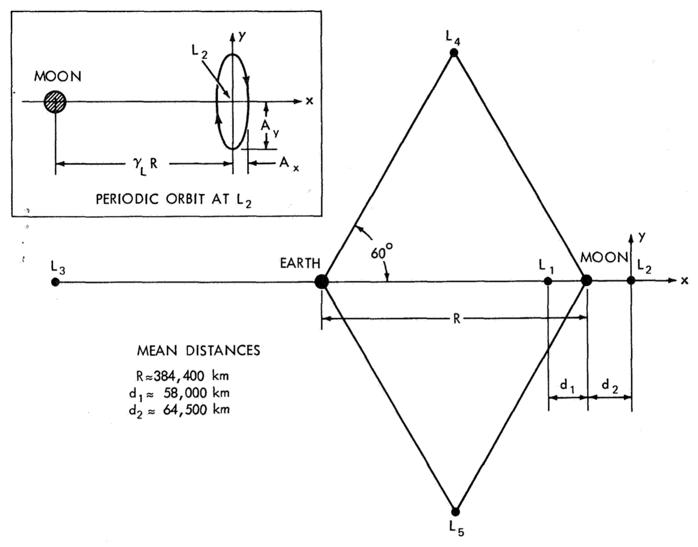
*Libration Points in the Earth-Moon System. From [Farquhar, 1971](https://www.lpi.usra.edu/lunar/documents/NASA%20TN%20D-6365.pdf).*
The Circular Restricted Three-Body Problem (CR3BP) is a continuing source of delight for astrodynamicists. If you think that, after 200 years, everything that could ever be written about this subject has already been written, you would be wrong. The basic premise is to describe the motion of a spacecraft in the vicinity of two celestial bodies that are in circular orbits about their common barycenter. The "restricted" part means that the spacecraft does not affect the motion of the other two bodies (i.e., its mass is negligible).
The normalized equations of motion for the CR3BP are very simple (see the Fortran Astrodynamics Toolkit):
subroutine crtbp_derivs(mu,x,dx)

implicit none

real(wp),intent(in) :: mu
!! CRTBP parameter
real(wp),dimension(6),intent(in) :: x
!! normalized state [r,v]
real(wp),dimension(6),intent(out) :: dx
!! normalized state derivative [rdot,vdot]

real(wp),dimension(3) :: r1,r2,rb1,rb2,r,v,g
real(wp) :: r13,r23,omm,c1,c2

r = x(1:3) ! position
v = x(4:6) ! velocity
omm = one - mu
rb1 = [-mu,zero,zero] ! location of body 1
rb2 = [omm,zero,zero] ! location of body 2
r1 = r - rb1 ! body1 -> sc vector
r2 = r - rb2 ! body2 -> sc vector
r13 = norm2(r1)**3
r23 = norm2(r2)**3
c1 = omm/r13
c2 = mu/r23

!normalized gravity from both bodies:
g(1) = -c1*(r(1) + mu) - c2*(r(1)-one+mu)
g(2) = -c1*r(2) - c2*r(2)
g(3) = -c1*r(3) - c2*r(3)

! derivative of x:
dx(1:3) = v ! rdot
dx(4) = two*v(2) + r(1) + g(1) ! vdot
dx(5) = -two*v(1) + r(2) + g(2) !
dx(6) = g(3) !

end subroutine crtbp_derivs
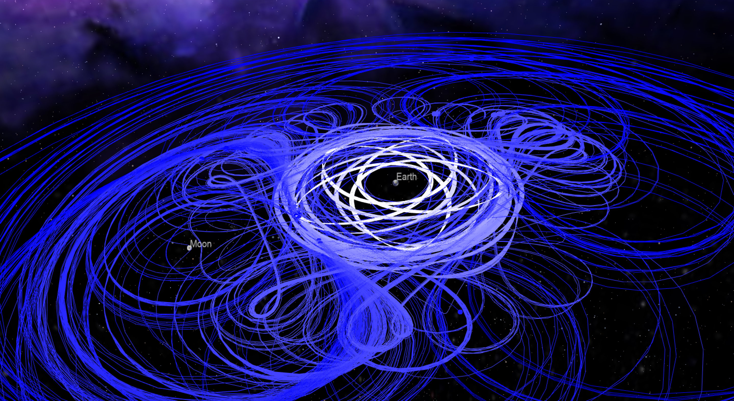
There are many types of interesting periodic orbits that exist in this system. I've mentioned Distant Retrograde Orbits (DROs) here before. Probably the most well-known CR3BP periodic orbits are called "halo orbits". Halo orbits can be computed in a similar manner as DROs (see previous post). For halos, we can get a good initial guess using an analytic approximation, and then use this guess to target the real thing. See the halo orbit module in the Fortran Astrodynamics Toolkit for an example of this approach. We can also use a continuation type method to generate families of orbits (say, for the L2 libration point, we have a range of halo orbits from near-planars that "orbit" L2, to near-rectilinears with close approaches to the secondary body). In a realistic force model (with the real ephemeris of the Earth, Moon, and Sun), the orbits generated using CR3BP assumptions are not periodic, but we can use the CR3BP solution as an initial guess in a multiple-shooting type approach with a numerical nonlinear equation solver to generate quasi-periodic multi-rev solutions. See the references below for details.
I generated the following image of a bunch of planar periodic CR3BP orbits using a program incorporating the Fortran Astrodynamics Toolkit and OpenFrames (an interface to the open source OpenSceneGraph library that can be used to visualize spacecraft trajectories). The initial states for the various orbits were taken from this database. Eventually, I will make this program open source when it is finished. There's also an online CR3BP propagator here.
See also
- M. Henon, "Numerical Exploration of the Restricted Problem. V. Hill’s Case: Periodic Orbits and Their Stability," Astronomy and Astrophys. Vol 1, 223-238, 1969.
- R. W. Farquhar, "The Utilization of Halo Orbits in Advanced Lunar Operation", NASA TN-D-6365, July 1971.
- D. L. Richardson, "Analytic Construction of Periodic Orbits About the Collinear Points", Celestial Mechanics 22 (1980)
- R. Mathur, C. A. Ocampo, "An Architecture for Incorporating Interactive Visualizations Into Scientific Simulations", 57th International Astronautical Congress, Valencia, Spain. IAC-06-D1.P.1.6.
- R. L. Restrepo, R. P. Russell, "A Database of Planar Axi-Symmetric Periodic Orbits for the Solar System," Paper AAS 17-694, AAS/AIAA Astrodynamics Specialist Conference, Stevenson, WA, Aug 2017.
- J. Williams, D. E. Lee, R. J. Whitley, K. A. Bokelmann, D. C. Davis, and C. F. Berry. "Targeting cislunar near rectilinear halo orbits for human space exploration", AAS 17-267
- Nabla Zero Labs, The Circular Restricted Three Body Problem.
- D. Davis, Near Rectilinear Halo Orbits Explained and Visualized, a.i. solutions, Jul 28, 2017 [YouTube]
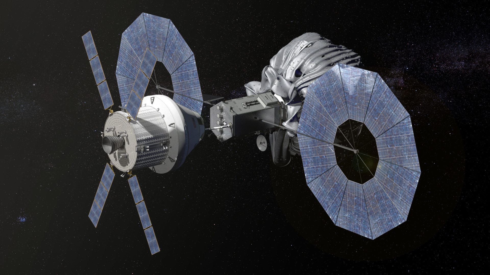
*Asteroid Redirect Mission [NASA]*
A "distant-retrograde orbit" (DRO) is a periodic orbit in the circular restricted three-body problem (CR3BP) that, in the rotating frame, looks like a large quasi-elliptical retrograde orbit around the secondary body. Moon-centered DRO's in the Earth-Moon system were considered as a possible destination for depositing a captured asteroid for NASA's proposed Asteroid Redirect Mission, since they can remain stable for long periods of time (decades or even centuries).
DROs can be computed using components from the Fortran Astrodynamics Toolkit. All we need is:
- A numerical integrator (we will use an 8th order Runge-Kutta method from Shanks [4]).
- The equations of motion for the circular restricted three-body problem (CR3BP).
- A nonlinear equation solver (we will use HYBRD1 from MINPACK).
We will use the canonical normalized CR3BP reference frame where the distance between the primary and secondary body is normalized to one. The initial state is placed on the x-axis, at a specified distance from the Moon. The y-velocity \(v_y\) is allowed to vary, and \(v_x=0\). The problem can be solved with two optimization variables:
- The time of flight for one orbit period (i.e., the duration between two consecutive x-axis crossings on the \(x>1\) side)
- The initial y-velocity component
and two constraints:
- \(y=0\) at the final time
- \(v_x=0\) at the final time (i.e., a perpendicular crossing of the x-axis)
The problem can be simplified to one variable and one constraint by using an integrator with an event-finding capability so that the integration proceeds until the x-axis crossing occurs (eliminating the time of flight and the \(y=0\) constraint from the optimization problem). That is how we will proceed here, since the Runge-Kutta module we are using does include an event location capability.
The code for computing a single Earth-Moon DRO is shown here:
program dro_test

    use fortran_astrodynamics_toolkit

    implicit none

    real(wp), parameter :: mu_earth = 398600.436233_wp
        !! km^3/s^2
    real(wp), parameter :: mu_moon = 4902.800076_wp
        !! km^3/s^2
    integer, parameter :: n = 6
        !! number of state variables
    real(wp), parameter :: t0 = 0.0_wp
        !! initial time (normalized)
    real(wp), parameter :: tmax = 1000.0_wp
        !! max final time (normalized)
    real(wp), parameter :: dt = 0.001_wp
        !! time step (normalized)
    real(wp), parameter :: xtol = 1.0e-4_wp
        !! tolerance for hybrd1
    integer, parameter :: maxfev = 1000
        !! max number of function evaluations for hybrd1
    real(wp), dimension(n), parameter :: x0 = &
                                         [1.2_wp, &
                                          0.0_wp, &
                                          0.0_wp, &
                                          0.0_wp, &
                                          -0.7_wp, &
                                          0.0_wp]
    !! initial guess for DRO state (normalized)

    real(wp), dimension(1) :: vy0
        !! initial y velocity (xvec for hybrd1)
    real(wp), dimension(1) :: vxf
        !! final x velocity (fvec for hybrd1)
    real(wp) :: mu
        !! CRTPB parameter
    type(rk8_10_class) :: prop
        !! integrator
    integer :: info
        !! hybrd1 status flag

    ! compute the CRTBP parameter & Jacobi constant:
    mu = compute_crtpb_parameter(mu_earth, mu_moon)

    ! initialize integrator:
    call prop%initialize(n, func, g=x_axis_crossing)

    ! now, solve for DRO:
    vy0 = x0(5) ! initial guess
    call hybrd1(dro_fcn, 1, vy0, vxf, tol=xtol, info=info)

    ! solution:
    write (*, *) ' info=', info
    write (*, *) ' vy0=', vy0
    write (*, *) ' vxf=', vxf

contains

!**************************************

    subroutine dro_fcn(n, xvec, fvec, iflag)
        !! DRO function for hybrd1

        implicit none

        integer, intent(in) :: n !! `n=1` in this case
        real(wp), dimension(n), intent(in) :: xvec !! `vy0`
        real(wp), dimension(n), intent(out) :: fvec !! `vxf`
        integer, intent(inout) :: iflag !! not used here

        real(wp) :: gf, t0, tf_actual
        real(wp), dimension(6) :: x, xf

        real(wp), parameter :: tol = 1.0e-8_wp
            !! event finding tolerance

        t0 = zero ! epoch doesn't matter for crtbp
        x = x0 ! initial guess state
        x(5) = xvec(1) ! vy0 (only optimization variable)

        !integrate to the next x-axis crossing:
        call prop%integrate_to_event(t0, x, dt, tmax, tol, tf_actual, xf, gf)

        !want x-velocity at the x-axis crossing to be zero:
        fvec = xf(4)

    end subroutine dro_fcn

!**************************************

    subroutine func(me, t, x, xdot)
        !! CRTBP derivative function

        implicit none

        class(rk_class), intent(inout) :: me
        real(wp), intent(in) :: t
        real(wp), dimension(me%n), intent(in) :: x
        real(wp), dimension(me%n), intent(out) :: xdot

        call crtbp_derivs(mu, x, xdot)

    end subroutine func

!**************************************

    subroutine x_axis_crossing(me, t, x, g)
        !! x-axis crossing event function

        implicit none

        class(rk_class), intent(inout) :: me
        real(wp), intent(in) :: t
        real(wp), dimension(me%n), intent(in) :: x
        real(wp), intent(out) :: g

        g = x(2) ! y = 0 at x-axis crossing

    end subroutine x_axis_crossing

end program dro_test
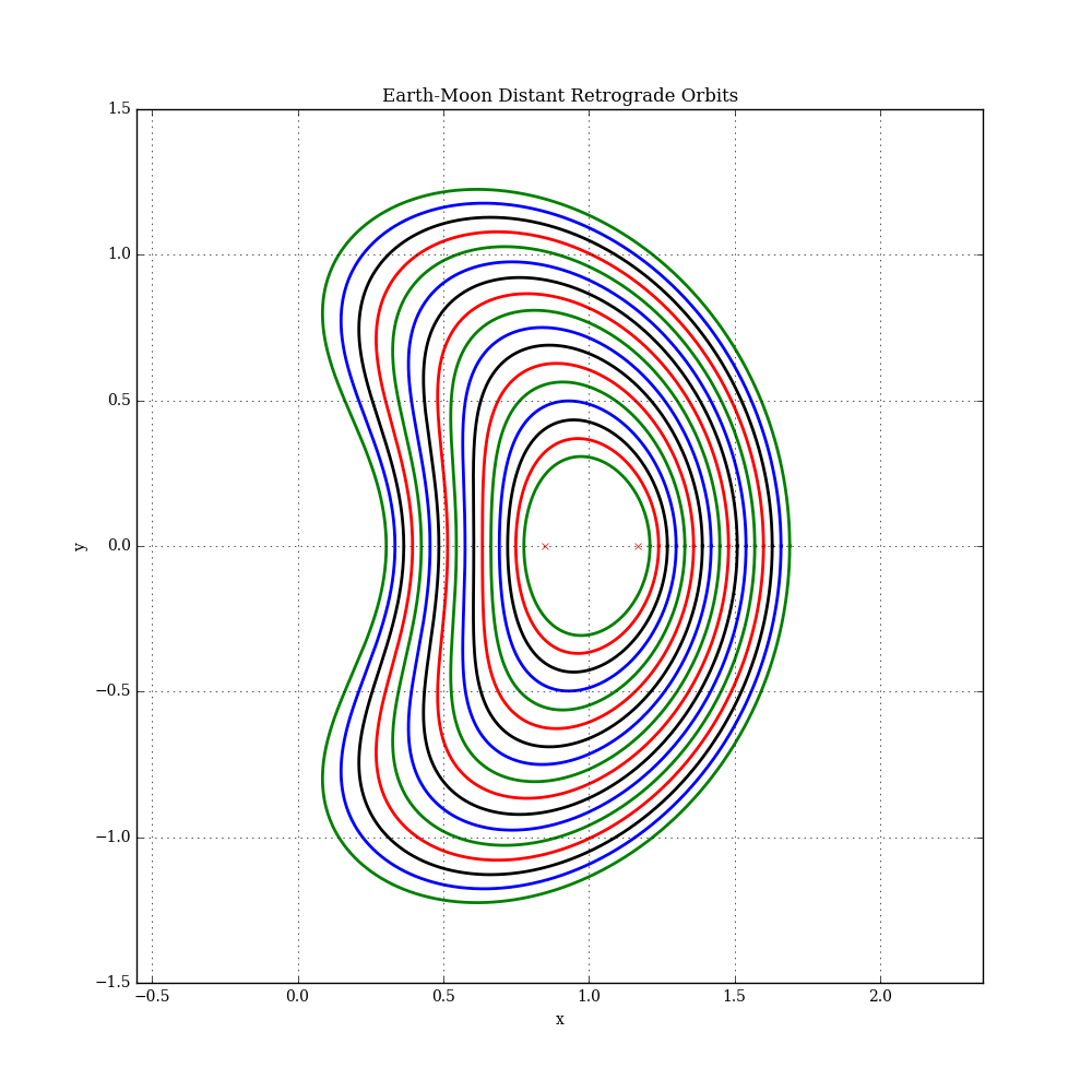
Trajectory plots for some example solutions are shown below (each with a different x component). The L1 and L2 libration points are also shown. In this plot, the Earth is at the origin and the Moon is at [x=1,y=0]. See this example for more details.
References
- The Restricted Three-Body Problem - MIT OpenCourseWare, S. Widnall 16.07 Dynamics Fall 2008, Version 1.0.
- C. A. Ocampo, G. W. Rosborough, "Transfer trajectories for distant retrograde orbiters of the Earth", AIAA Spaceflight Mechanics Meeting, Pasadena, CA, Feb. 22-24, 1993.
- Asteroid Redirect Mission and Human Space Flight, June 19, 2013.
- E. B. Shanks, "Higher Order Approximations of Runge-Kutta Type", NASA Technical Note, NASA TN D-2920, Sept. 1965.
- Henon, M., "Numerical Exploration of the Restricted Problem. V. Hill's Case: Periodic Orbits and Their Stability," Astronomy and Astrophys. Vol 1, 223-238, 1969.