Degenerate Conic

Near Rectilinear Halo Orbits

nrhos

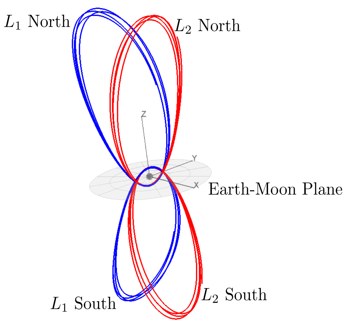
Some Earth-Moon NRHOs. From Williams et al, 2017.

I have mentioned the Circular Restricted Three-Body Problem (CR3BP) here a couple of times. Another type of periodic CR3BP orbit is the "near rectilinear" halo orbit (NRHO). These orbits are just the continuation of the family of "normal" halo orbits until they get very close to the secondary body [1]. Like all halo orbits, there are "northern" and "southern" families (see image above). NASA chose a lunar L2 NRHO (southern family, which spends more time over the lunar South pole) as the destination orbit for the Deep Space Gateway [2]. The CAPSTONE mission [3] successfully launched on June 28, 2022, and is currently en route to the Gateway NRHO. [4-5]

Computing an NRHO

A basic NRHO in the CR3BP can be computed just like a "normal" halo orbit. (see this and this earlier post). In Reference [2] we described methods for generating long-duration NRHOs in a realistic force model. The procedure involves a multiple shooting method using the CR3BP solution as an initial guess replicated for multiple revs of the orbit. Then a simple nonlinear solver is used to impose state and time continuity for the full orbit.

All we need to start the process is an initial guess. Appendix A.1 in Reference [6] lists a table of CR3BP Earth-Moon L2 halo orbits. An example NRHO from this table is shown here:

Parameter	Value
\(l^{*}\)	384400.0
\(t^{*}\)	375190.25852
Jacobi constant	3.0411
period	1.5872714606
\(x_0\)	1.0277926091
\(z_0\)	-0.1858044184
\(\dot y_0\)	-0.1154896637

In this table, the three state parameters (\(x_0\), \(z_0\), and \(\dot y_0\)) are given in the canonical normalized CR3BP system, with respect to the Earth-Moon barycenter. The distance and time normalization factors (\(l^{*}\) and \(t^{*}\)) can be used to convert them into normal distance and time units (km and sec).

The process is fairly straightforward, and is demonstrated in a new tool, which I call Halo. It is written in Modern Fortran. The Halo tool uses the initial CR3BP state to generate a long-duration orbit in the real ephemeris model. Halo doesn't use the CR3BP equations of motion, since we will be integrating in the real system, using the actual ephemeris of the Earth and Moon, and so we use the real units. See Reference [7] for some further details about an earlier version of this code. Halo is built upon a number of open source Fortran libraries, and the main components of the tool are:

General astrodynamics routines, including: ephemeris of the Sun, Earth, and Moon, a spherical harmonic lunar gravity model, state transformations, etc. These are all provided by the Fortran Astrodynamics Toolkit.
A numerical integration method. I'm using DDEABM, which is an Adams method. I like this method, which has a long heritage and seems to have a good balance of speed and accuracy for these kinds of astrodynamics problems.
A way to compute derivatives, which are needed by the solver for the Jacobian. For this problem, finite-difference numerical derivatives are good enough, so I'm using my NumDiff library. Since the problem ends up being quite sparse, we can use the NumDiff options to quickly compute the Jacobian matrix by taking into account the sparsity pattern.
A nonlinear numerical solver. I'm using my nlsolver-fortran library. The problem being solved is "underdetermined", meaning there are more free variables than there are constraints. Nlsolver-Fortran can solve these problems just fine using a basic Newton-type minimum norm method. In astrodynamics, you will usually see this type of method called a "differential corrector".

Halo makes use of the amazing Fortran Package Manager (FPM) for dependency management and compilation. In the fpm.toml manifest file, all we have to do is specify the dependencies like so:

[dependencies]
fortran-astrodynamics-toolkit = { git = "https://github.com/jacobwilliams/Fortran-Astrodynamics-Toolkit", tag = "0.4" }
NumDiff = { git = "https://github.com/jacobwilliams/NumDiff", tag = "1.5.1" }
ddeabm = { git = "https://github.com/jacobwilliams/ddeabm", tag = "3.0.0" }
json-fortran = { git = "https://github.com/jacobwilliams/json-fortran", tag = "8.2.5" }
bspline-fortran = { git = "https://github.com/jacobwilliams/bspline-fortran", tag = "6.1.0" }
pyplot-fortran = { git = "https://github.com/jacobwilliams/pyplot-fortran", tag = "3.2.0" }
fortran-search-and-sort = { git = "https://github.com/jacobwilliams/fortran-search-and-sort", tag = "1.0.0" }
fortran-csv-module = { git = "https://github.com/jacobwilliams/fortran-csv-module", tag = "1.3.0" }
nlesolver-fortran = { git = "https://github.com/jacobwilliams/nlesolver-fortran", tag = "1.0.0" }
argv-fortran = { git = "https://github.com/jacobwilliams/argv-fortran", tag = "1.0.0" }

libs-for-halo

FPM will download the specified versions of everything and build the tool with a single command like so:

fpm build --profile release

This is really a game changer for Fortran. Before FPM, poor Fortran users had no package manager at all. A common anti-pattern was to manually download code from somewhere like Netlib and then manually add the files to your repo and manually edit your makefiles to incorporate it into your compile process. This is literally what SciPy has done, and now they have forks of all their Fortran code that just lives inside the SciPy monorepo, with no way to distribute it upstream to the original library source, or downstream to other Fortran codes that might want to use it. FPM makes it all just effortless to specify dependencies (and update the version numbers if the upstream code changes) and finally allows and encourages Fortran users to develop a modern system of interdependent libraries with sane and modern version control practices.

Example

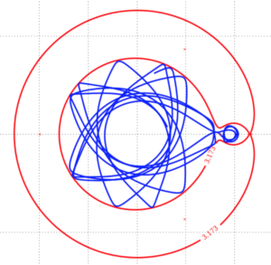
Using the initial guess from the table above, we can use Halo to compute a ballistic NRHO for 50 revs (about 344 days for this example) in the real ephemeris model. The 50 rev problem has 1407 control variables and 1200 equality constraints. Convergence takes about 31 seconds (6 iterations of the solver) on my M1 MacBook Pro, complied using the Intel Fortran compiler:

Iteration number	norm2(Constraint violation vector)
1	0.2936000870578949
2	0.1554308242228055
3	0.0611200979653433
4	0.0052758762761737
5	0.0000031933098398
6	0.0000000035186120

nrho_solution

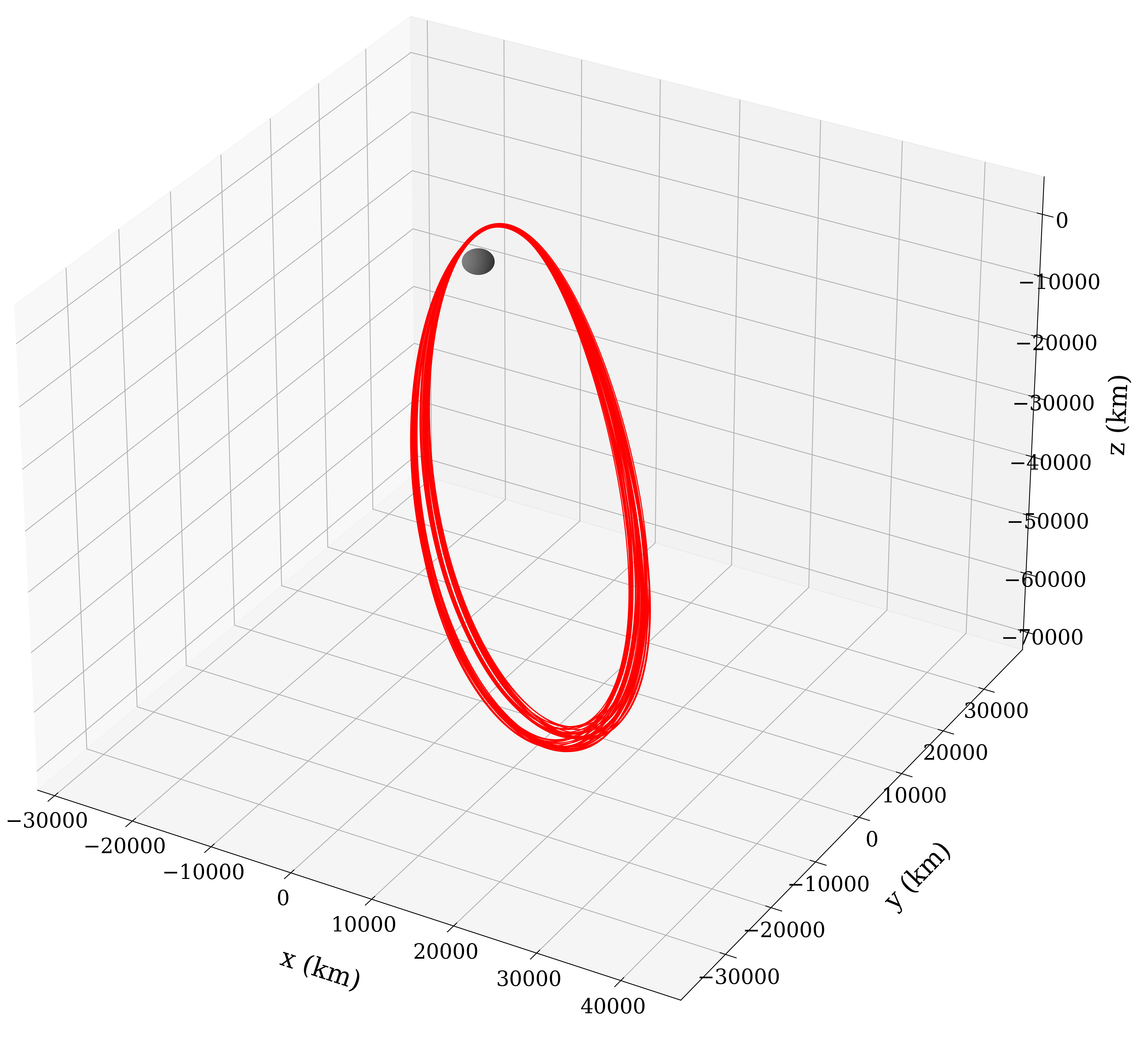
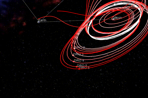
50 Rev NRHO Solution. Visualized here in the Moon-centered Earth-Moon rotating frame.

There's no parallelization currently being used here, so there are some opportunities to speed it up even more. In Reference [2] we also show how the above procedure can be used to kick off a "receding horizon" approach to compute even longer duration NRHOs that include very small correction burns. This is the process that was used to generate the Gateway orbit [4-5], and the Halo program could be updated to do that as well. But that is a post for another time.

Circular Restricted Three-Body Problem

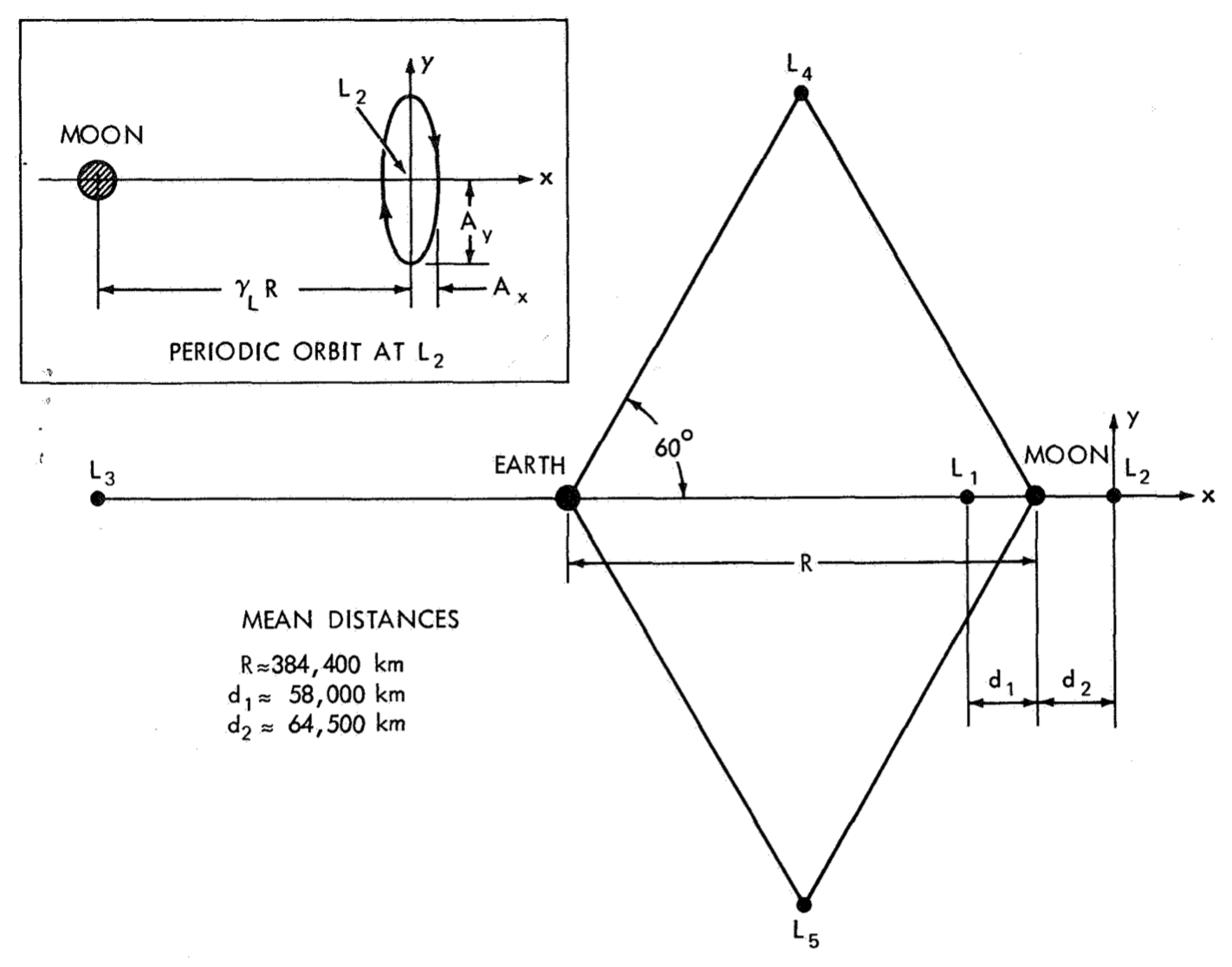
Libration Points in the Earth-Moon System. From Farquhar, 1971.

The Circular Restricted Three-Body Problem (CR3BP) is a continuing source of delight for astrodynamicists. If you think that, after 200 years, everything that could ever be written about this subject has already been written, you would be wrong. The basic premise is to describe the motion of a spacecraft in the vicinity of two celestial bodies that are in circular orbits about their common barycenter. The "restricted" part means that the spacecraft does not affect the motion of the other two bodies (i.e., its mass is negligible).

The normalized equations of motion for the CR3BP are very simple (see the Fortran Astrodynamics Toolkit):

subroutine crtbp_derivs(mu,x,dx)

implicit none

real(wp),intent(in) :: mu
!! CRTBP parameter
real(wp),dimension(6),intent(in) :: x
!! normalized state [r,v]
real(wp),dimension(6),intent(out) :: dx
!! normalized state derivative [rdot,vdot]

real(wp),dimension(3) :: r1,r2,rb1,rb2,r,v,g
real(wp) :: r13,r23,omm,c1,c2

r = x(1:3) ! position
v = x(4:6) ! velocity
omm = one - mu
rb1 = [-mu,zero,zero] ! location of body 1
rb2 = [omm,zero,zero] ! location of body 2
r1 = r - rb1 ! body1 -> sc vector
r2 = r - rb2 ! body2 -> sc vector
r13 = norm2(r1)**3
r23 = norm2(r2)**3
c1 = omm/r13
c2 = mu/r23

!normalized gravity from both bodies:
g(1) = -c1*(r(1) + mu) - c2*(r(1)-one+mu)
g(2) = -c1*r(2) - c2*r(2)
g(3) = -c1*r(3) - c2*r(3)

! derivative of x:
dx(1:3) = v ! rdot
dx(4) = two*v(2) + r(1) + g(1) ! vdot
dx(5) = -two*v(1) + r(2) + g(2) !
dx(6) = g(3) !

end subroutine crtbp_derivs

There are many types of interesting periodic orbits that exist in this system. I've mentioned Distant Retrograde Orbits (DROs) here before. Probably the most well-known CR3BP periodic orbits are called "halo orbits". Halo orbits can be computed in a similar manner as DROs (see previous post). For halos, we can get a good initial guess using an analytic approximation, and then use this guess to target the real thing. See the halo orbit module in the Fortran Astrodynamics Toolkit for an example of this approach. We can also use a continuation type method to generate families of orbits (say, for the L2 libration point, we have a range of halo orbits from near-planars that "orbit" L2, to near-rectilinears with close approaches to the secondary body). In a realistic force model (with the real ephemeris of the Earth, Moon, and Sun), the orbits generated using CR3BP assumptions are not periodic, but we can use the CR3BP solution as an initial guess in a multiple-shooting type approach with a numerical nonlinear equation solver to generate quasi-periodic multi-rev solutions. See the references below for details.

I generated the following image of a bunch of planar periodic CR3BP orbits using a program incorporating the Fortran Astrodynamics Toolkit and OpenFrames (an interface to the open source OpenSceneGraph library that can be used to visualize spacecraft trajectories). The initial states for the various orbits were taken from this database. Eventually, I will make this program open source when it is finished. There's also an online CR3BP propagator here.

screenshot5

Low Lunar Orbit Maintenance

Altair's ascent stage docking with Orion [NASA]

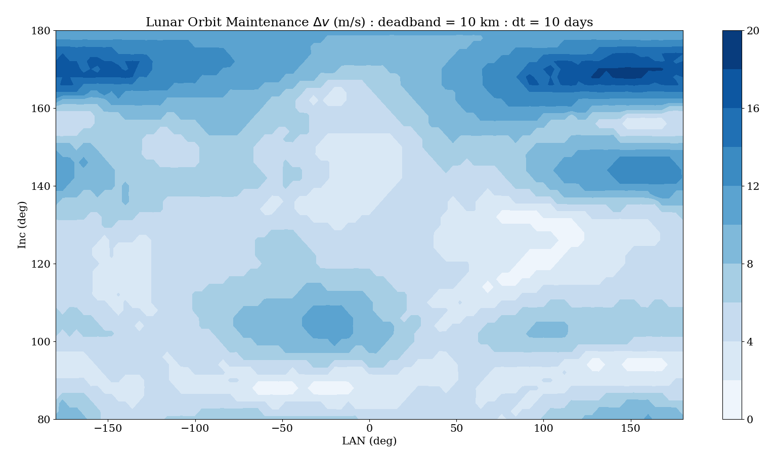
The lunar gravity field is bumpy. Thus a spacecraft in a low lunar orbit for an extended period of time must perform periodic correction maneuvers or the orbit eventually becomes unstable and can crash into the Moon. When the Orion spacecraft was being designed during the late Constellation Program, the requirements of global surface access sortie missions, six-month polar outpost missions, anytime aborts, and autonomous operation of the vehicle while the crew was on the surface, required lots of analysis to figure out how to make the architecture work. And then the program was canceled.

The reference low-lunar orbit maintenance algorithm we used during Constellation was fairly simple. Orion initially inserted into a retrograde circular parking orbit with a 100 km altitude. During orbit propagation, if the altitude was reduced by a specified deadband altitude (say 10 km) the vehicle would perform a periapsis raise maneuver at the next apoapsis to bring the periapsis back up to 100 km. The apoapsis radius was not controlled, and indeed all the other orbital elements were also allowed to float. This would continue until the crew was ready to return (on the Altiar lander ascent stage), at which point Orion would circularize the orbit and perform a plane change to allow Altair to perform an in-plane ascent.

The \(\Delta v\) maneuver to perform at apoapsis of an orbit with a periapsis radius \(r_{pi}\) and apoapsis radius \(r_{ai}\), to target a periapsis radius \(r_{pf}\) can be computed by:

Initial apoapsis velocity: \(v_{ai} = \sqrt{ 2 \mu \frac{r_{pi}}{r_{ai} (r_{ai}+r_{pi})} }\)
Final apoapsis velocity: \(v_{af} = \sqrt{ 2 \mu \frac{r_{pf}}{r_{ai} (r_{ai}+r_{pf})} }\)
Maneuver magnitude: \(\Delta v = v_{af} - v_{ai}\)

We can implement this method using the Fortran Astrodynamics Toolkit fairly easily. We also need an integrator with an event finding capability (we can use DDEABM, a variable step size variable order Adams method). We propagate from the initial insertion state until the deadband altitude is violated, then propagate to the next apoapsis where the periapsis raise maneuver is performed, then repeat as necessary. The code implementing this scheme can be found on GitHub here. For the force model, we are using a 20 x 20 GRAIL geopotential model of the Moon (not available during Constellation, when we used the Lunar Prospector derived LP150Q model). A contour plot of the results for 100 km retrograde orbits with a 10 km altitude deadband and 10 days of propagation time are shown below. Each maneuver ends up being about 2 m/s for this example, and the bumpiness of the gravity field is evident. Some insertion orbits require no maneuvers, while others require about 18 m/s over the 10 day period.

lom

New Coordinate Systems for Solar System Bodies

ann18010a

The International Astronomical Union (IAU) has published a new report with their latest recommendations for the cartographic coordinates and rotational elements of planetary bodies. The new guidelines, equations, and coefficients have been updated based on the latest data (including from interplanetary missions such as MESSENGER, Dawn, Rosetta, and Stardust-NExT).

One difference from the previous reports is that the low-fidelity Earth and Moon frames have been removed "in order to avoid confusion", since high-accuracy Earth and Moon frames are available. I mentioned the IAU_EARTH and IAU_MOON frames in a previous post. They are available in SPICE and the Fortran Astrodynamics Toolkit. I think it's unfortunate that they were removed. It's true that these are not ultra-precise frames (see, for example, this tutorial from JPL). However, low-to-medium fidelity frames are still very useful for many applications, including spacecraft trajectory optimization. A frame that is good enough, is very fast to compute, is continuous and differentiable for all time, and can be implemented in a few lines of code is often preferable to having to deal with thousands of lines of SOFA or SPICE code, leap second confusion, binary kernel files, etc. that are required to get the high-accuracy frames to work.

Orbital Mechanics with Fortran

crtbp

Many of NASA's workhorse spacecraft trajectory optimization tools are written in Fortran or have Fortran components (e.g., OTIS, MALTO, Mystic, and Copernicus). None of it is really publicly-available however. There are some freely-available Fortran codes around for general-purpose orbital mechanics applications. Including:

Fortran Astrodynamics Toolkit — A Modern Fortran Library for Astrodynamics. This is my hobby library that is coming along nicely, and includes a lot of different algorithms. See also my other GitHub projects for other components that are useful in the orbital mechanics field (such as integrators and optimizers). All of it is open source with a permissive BSD license (so you can use it for whatever you want).
Low-Level Engine for Astrodynamics (LLEA) another modern Fortran astrodynamics library on GitHub
Astrodynamics Software from Fundamentals of Astrodynamics and Applications by David Vallado
Orbital Mechanics with Fortran by Dave Eagle
IAU Standards of Fundamental Astronomy (SOFA)
Naval Observatory Vector Astrometry Software (NOVAS)
SPICE Toolkit from JPL/NAIF for solar system geometry
Swifter — an improved solar system integration software package

You can also find some old Fortran gems in various papers on the NASA Technical Reports Server.

Distant Retrograde Orbits

Asteroid Redirect Mission

Asteroid Redirect Mission [NASA]

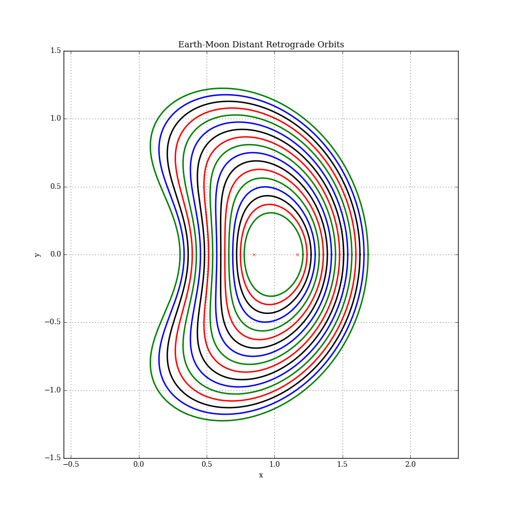
A "distant-retrograde orbit" (DRO) is a periodic orbit in the circular restricted three-body problem (CR3BP) that, in the rotating frame, looks like a large quasi-elliptical retrograde orbit around the secondary body. Moon-centered DRO's in the Earth-Moon system were considered as a possible destination for depositing a captured asteroid for NASA's proposed Asteroid Redirect Mission, since they can remain stable for long periods of time (decades or even centuries).

DROs can be computed using components from the Fortran Astrodynamics Toolkit. All we need is:

A numerical integrator (we will use an 8th order Runge-Kutta method from Shanks [4]).
The equations of motion for the circular restricted three-body problem (CR3BP).
A nonlinear equation solver (we will use HYBRD1 from MINPACK).

We will use the canonical normalized CR3BP reference frame where the distance between the primary and secondary body is normalized to one. The initial state is placed on the x-axis, at a specified distance from the Moon. The y-velocity \(v_y\) is allowed to vary, and \(v_x=0\). The problem can be solved with two optimization variables:

The time of flight for one orbit period (i.e., the duration between two consecutive x-axis crossings on the \(x>1\) side)
The initial y-velocity component

and two constraints:

\(y=0\) at the final time
\(v_x=0\) at the final time (i.e., a perpendicular crossing of the x-axis)

The problem can be simplified to one variable and one constraint by using an integrator with an event-finding capability so that the integration proceeds until the x-axis crossing occurs (eliminating the time of flight and the \(y=0\) constraint from the optimization problem). That is how we will proceed here, since the Runge-Kutta module we are using does include an event location capability.

The code for computing a single Earth-Moon DRO is shown here:

program dro_test

    use fortran_astrodynamics_toolkit

    implicit none

    real(wp), parameter :: mu_earth = 398600.436233_wp
        !! km^3/s^2
    real(wp), parameter :: mu_moon = 4902.800076_wp
        !! km^3/s^2
    integer, parameter :: n = 6
        !! number of state variables
    real(wp), parameter :: t0 = 0.0_wp
        !! initial time (normalized)
    real(wp), parameter :: tmax = 1000.0_wp
        !! max final time (normalized)
    real(wp), parameter :: dt = 0.001_wp
        !! time step (normalized)
    real(wp), parameter :: xtol = 1.0e-4_wp
        !! tolerance for hybrd1
    integer, parameter :: maxfev = 1000
        !! max number of function evaluations for hybrd1
    real(wp), dimension(n), parameter :: x0 = &
                                         [1.2_wp, &
                                          0.0_wp, &
                                          0.0_wp, &
                                          0.0_wp, &
                                          -0.7_wp, &
                                          0.0_wp]
    !! initial guess for DRO state (normalized)

    real(wp), dimension(1) :: vy0
        !! initial y velocity (xvec for hybrd1)
    real(wp), dimension(1) :: vxf
        !! final x velocity (fvec for hybrd1)
    real(wp) :: mu
        !! CRTPB parameter
    type(rk8_10_class) :: prop
        !! integrator
    integer :: info
        !! hybrd1 status flag

    ! compute the CRTBP parameter & Jacobi constant:
    mu = compute_crtpb_parameter(mu_earth, mu_moon)

    ! initialize integrator:
    call prop%initialize(n, func, g=x_axis_crossing)

    ! now, solve for DRO:
    vy0 = x0(5) ! initial guess
    call hybrd1(dro_fcn, 1, vy0, vxf, tol=xtol, info=info)

    ! solution:
    write (*, *) ' info=', info
    write (*, *) ' vy0=', vy0
    write (*, *) ' vxf=', vxf

contains

!**************************************

    subroutine dro_fcn(n, xvec, fvec, iflag)
        !! DRO function for hybrd1

        implicit none

        integer, intent(in) :: n !! `n=1` in this case
        real(wp), dimension(n), intent(in) :: xvec !! `vy0`
        real(wp), dimension(n), intent(out) :: fvec !! `vxf`
        integer, intent(inout) :: iflag !! not used here

        real(wp) :: gf, t0, tf_actual
        real(wp), dimension(6) :: x, xf

        real(wp), parameter :: tol = 1.0e-8_wp
            !! event finding tolerance

        t0 = zero ! epoch doesn't matter for crtbp
        x = x0 ! initial guess state
        x(5) = xvec(1) ! vy0 (only optimization variable)

        !integrate to the next x-axis crossing:
        call prop%integrate_to_event(t0, x, dt, tmax, tol, tf_actual, xf, gf)

        !want x-velocity at the x-axis crossing to be zero:
        fvec = xf(4)

    end subroutine dro_fcn

!**************************************

    subroutine func(me, t, x, xdot)
        !! CRTBP derivative function

        implicit none

        class(rk_class), intent(inout) :: me
        real(wp), intent(in) :: t
        real(wp), dimension(me%n), intent(in) :: x
        real(wp), dimension(me%n), intent(out) :: xdot

        call crtbp_derivs(mu, x, xdot)

    end subroutine func

!**************************************

    subroutine x_axis_crossing(me, t, x, g)
        !! x-axis crossing event function

        implicit none

        class(rk_class), intent(inout) :: me
        real(wp), intent(in) :: t
        real(wp), dimension(me%n), intent(in) :: x
        real(wp), intent(out) :: g

        g = x(2) ! y = 0 at x-axis crossing

    end subroutine x_axis_crossing

end program dro_test

Trajectory plots for some example solutions are shown below (each with a different x component). The L1 and L2 libration points are also shown. In this plot, the Earth is at the origin and the Moon is at [x=1,y=0]. See this example for more details.

dros

References

The Restricted Three-Body Problem - MIT OpenCourseWare, S. Widnall 16.07 Dynamics Fall 2008, Version 1.0.
C. A. Ocampo, G. W. Rosborough, "Transfer trajectories for distant retrograde orbiters of the Earth", AIAA Spaceflight Mechanics Meeting, Pasadena, CA, Feb. 22-24, 1993.
Asteroid Redirect Mission and Human Space Flight, June 19, 2013.
E. B. Shanks, "Higher Order Approximations of Runge-Kutta Type", NASA Technical Note, NASA TN D-2920, Sept. 1965.
Henon, M., "Numerical Exploration of the Restricted Problem. V. Hill's Case: Periodic Orbits and Their Stability," Astronomy and Astrophys. Vol 1, 223-238, 1969.

posted at 19:49 · Orbital Mechanics · DRO Fortran

SOFA

The Standards of Fundamental Astronomy (SOFA) library is a very nice collection of routines that implement various IAU algorithms for fundamental astronomy computations. Versions are available in Fortran and C. Unfortunately, the Fortran version is written to be of maximum use to astronomers who frequently travel back in time to 1977 and compile the code on their UNIVAC (i.e., it is fixed-format Fortran 77). To assist 21st century users, I uploaded a little Python script called SofaMerge to Github. This script can make your life easier by merging all the individual source files into a single Fortran module file (with a few cosmetic updates along the way). It doesn't yet include any fixed to free format changes, but that could be easily added later.

posted at 02:06 · Orbital Mechanics · C Fortran IAU Python Orbital Mechanics SOFA

Speeding up SPICE

The SPICE Toolkit software is an excellent package of very well-written and well-documented routines for a variety of astrodynamics applications. It is produced by NASA's Navigation and Ancillary Information Facility (NAIF). Versions are available for Fortran 77, C, IDL, and Matlab.

To speed up the execution of SPICE-based programs, there are a few things you can do:

For the Fortran SPICELIB, recompile it with optimization enabled (say, -O2). The default library released by NAIF is not compiled with optimization.
Turn off the SPICE traceback system (call TRCOFF()). If you are using a compiler that has a built-in stack trace routine (for example TRACEBACKQQ in the Intel compiler), just include a call to it in the SPICE BYEBYE.F routine. That will give you a stack trace for any fatal errors.
Converting a non-native binary PCK to native form will also speed up data access somewhat.
Calls to ephemeris routines where the target and observer bodies are input as strings will be slightly slower than the ones where the inputs are the NAIF ID codes (which are integers). For example, for the geometric state (position and velocity) of one body relative to another, use SPKGEO instead of SPKEZR. Also, if all you require is position and not velocity, use SPKGPS instead of SPKGEO, since it will be a bit faster.

Also note that for applications only requiring the ephemerides of the solar system major bodies, there is an older code from JPL (PLEPH) which is simpler and faster than SPICE, but uses a different format for the ephemeris files.

posted at 21:24 · Orbital Mechanics · Fortran Orbital Mechanics SPICE

Porkchop Plots

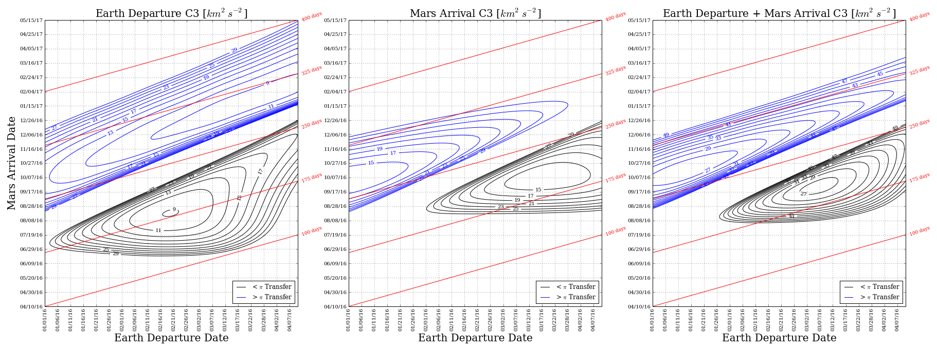
A porkchop plot is a data visualization tool used in interplanetary mission design which displays contours of various quantities as a function of departure and arrival date. Example pork chop plots for 2016 Earth-Mars transfers are shown here. The x-axis is the Earth departure date, and the y-axis is the Mars arrival date. The contours show the Earth departure C3, the Mars arrival C3, and the sum of the two. C3 is the "characteristic energy" of the departure or arrival, and is equal to the \(v_{\infty}^2\) of the hyperbolic trajectory. Each point on the curve represents a ballistic Earth-Mars transfer (computed using a Lambert solver). The two distinct black and blue contours on each plot represent the "short way" (\(<\pi\)) and "long way" (\(>\pi\)) transfers. The contours look vaguely like pork chops, the centers being the lowest C3 value, and thus optimal transfers. The January - October 2016 opportunity will be used for the ExoMars Trace Gas Orbiter, and the March - September 2016 opportunity will be used for InSight.

References

A. B. Sergeyevsky, G. C. Snyder, R. A. Cunniff, "Interplanetary Mission Design Handbook, Volume I, Part 2: Earth to Mars Ballistic Mission Opportunities, 1990-2005", NASA JPL, September 1983.
L. M. Burke, R. D. Falck, and M. L. McGuire, "Interplanetary Mission Design Handbook: Earth-to-Mars Mission Opportunities 2026 to 2045", NASA/TM—2010-216764, October 2010.
Chauncey Uphoff, The History of the Term C3, 2001.

posted at 00:13 · Orbital Mechanics · C3 Lambert Mars Orbital Mechanics

Algorithms • Modern Fortran Programming • Orbital Mechanics

Jul 31, 2022

Near Rectilinear Halo Orbits

Computing an NRHO

Example

See also

Aug 05, 2018

Circular Restricted Three-Body Problem

See also

May 06, 2018

Low Lunar Orbit Maintenance

See also

Apr 15, 2018

New Coordinate Systems for Solar System Bodies

See also

Apr 04, 2018

Orbital Mechanics with Fortran

See also

May 15, 2016

Distant Retrograde Orbits

References

Jan 29, 2015

SOFA

Dec 20, 2014

Speeding up SPICE

Nov 09, 2014

Porkchop Plots

References