Jul 13, 2014
I'm starting a new project on GitHub: the Fortran Astrodynamics Toolkit. Hardly anyone is developing open source orbital mechanics software for modern Fortran, so the time has come. Most of the code from this blog will eventually find its way there. My goal is to include modern Fortran implementations of all the standard orbital mechanics algorithms such as:
- Lambert solvers
- Kepler propagators
- ODE solvers (Runge-Kutta, Nyström, Adams)
- Orbital element conversions
Then we'll see where it goes from there. The code will be released under a permissive BSD style license.
Jul 08, 2014
Here is a simple Fortran subroutine to return only the unique values in a vector (inspired by Matlab's unique function). Note, this implementation is for integer arrays, but could easily be modified for any type. This code is not particularly optimized, so there may be a more efficient way to do it. It does demonstrate Fortran array transformational functions such as pack and count. Note that to duplicate the Matlab function, the output array must also be sorted.
subroutine unique(vec,vec_unique)
! Return only the unique values from vec.

implicit none

integer,dimension(:),intent(in) :: vec
integer,dimension(:),allocatable,intent(out) :: vec_unique

integer :: i,num
logical,dimension(size(vec)) :: mask

mask = .false.

do i=1,size(vec)

    !count the number of occurrences of this element:
    num = count( vec(i)==vec )

    if (num==1) then
        !there is only one, flag it:
        mask(i) = .true.
    else
        !flag this value only if it hasn't already been flagged:
        if (.not. any(vec(i)==vec .and. mask) ) mask(i) = .true.
    end if

end do

!return only flagged elements:
allocate( vec_unique(count(mask)) )
vec_unique = pack( vec, mask )

!if you also need it sorted, then do so.
! For example, with slatec routine:
!call ISORT (vec_unique, [0], size(vec_unique), 1)

end subroutine unique
Jul 08, 2014
I agree with everything said in this article: My Corner of the World: C++ vs Fortran. I especially like the bit contrasting someone trying to learn C++ for the first time in order to do some basic linear algebra (like a matrix multiplication). Of course, in Fortran, this is a built-in part of the language:
matrix_c = matmul(matrix_a, matrix_b)
Whereas, for C++:
The bare minimum for doing the same exercise in C++ is that you have to get your hands on a library that does what you want. So you have to know about the existence of Eigen or another library. Then you have to figure out how to call it. Then you have to figure out how to link to an external library. And the documentation is probably not that helpful. There are friendly C++ users for sure. It's just that you won't have a clue what they're telling you to do. They'll be telling you to set up a makefile. They'll be recommending that you look at Boost and talking about how great it is and you'll be all WTF.
And before you use that C++ library, are you really sure you won't end up with a memory leak? Do you even know what a memory leak is?
Jul 06, 2014
In the last few years, a number of excellent books have been published about modern Fortran:
- R. J. Hanson, Numerical Computing With Modern Fortran, SIAM-Society for Industrial and Applied Mathematics, 2013.
- A. Markus, Modern Fortran in Practice, Cambridge University Press, 2012.
- M. Metcalf, J. Reid, M. Cohen, Modern Fortran Explained, Oxford University Press, 2011.
- N. S. Clerman, W. Spector, Modern Fortran: Style and Usage, Cambridge University Press, 2011.
In addition, other more general-purpose references on modern programming concepts (such as object-oriented programming and high performance computing) tailored to the Fortran programmer are:
- D. Rouson, J. Xia, X. Xu, Scientific Software Design: The Object-Oriented Way, Cambridge University Press, 2011.
- G. Hager, G. Wellein, Introduction to High Performance Computing for Scientists and Engineers, CRC Press, 2011.
All of these are highly recommended, especially if you want to learn modern Fortran for the first time. Under no circumstances should you purchase any Fortran book with the numbers "77", "90", or "95" in the title.
Jul 05, 2014
Updated July 7, 2014
Poorly commented sourcecode is one of my biggest pet peeves. Not only should the comments explain what the routine does, but where the algorithm came from and what its limitations are. Consider ISORT, a non-recursive quicksort routine from SLATEC, written in 1976. In it, we encounter the following code:
R = 0.375E0
...
IF (R .LE. 0.5898437E0) THEN
    R = R+3.90625E-2
ELSE
    R = R-0.21875E0
ENDIF
What are these magic numbers? An internet search for "0.5898437" yields dozens of hits, many of them different versions of this algorithm translated into various other programming languages (including C, C++, and free-format Fortran). Note: the algorithm here is the same one, but also prefaces this code with the following helpful comment:
! And now...Just a little black magic...
Frequently, old code originally written in single precision can be improved on modern computers by updating to full-precision constants (replacing 3.14159 with a parameter computed at compile time as acos(-1.0_wp) is a classic example). Is this the case here? Sometimes WolframAlpha is useful in these circumstances. It tells me that a possible closed form of 0.5898437 is: \(\frac{57}{100\pi}+\frac{13\pi}{100} \approx 0.58984368009\). Hmmmmm... The reference given in the header is no help [1], it doesn't contain this bit of code at all.
It turns out, what this code is doing is generating a pseudorandom number to use as the pivot element in the quicksort algorithm. The code produces the following repeating sequence of values for R:
0.375
0.4140625
0.453125
0.4921875
0.53125
0.5703125
0.609375
0.390625
0.4296875
0.46875
0.5078125
0.546875
0.5859375
0.625
0.40625
0.4453125
0.484375
0.5234375
0.5625
0.6015625
0.3828125
0.421875
0.4609375
0.5
0.5390625
0.578125
0.6171875
0.3984375
0.4375
0.4765625
0.515625
0.5546875
0.59375
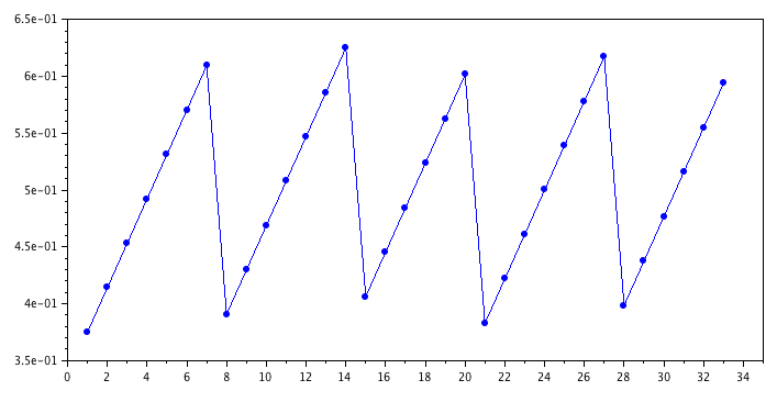
This places the pivot point near the middle of the set. The source of this scheme is from Reference [2], and is also mentioned in Reference [3]. According to [2]:
These four decimal constants, which are respectively 48/128, 75.5/128, 28/128, and 5/128, are rather arbitrary.
The other magic numbers in this routine are the dimensions of these variables:
These are workspace arrays used by the subroutine, since it does not employ recursion. But, since they have a fixed size, there is a limit to the size of the input array this routine can sort. What is that limit? You would not know from the documentation in this code. You have to go back to the original reference [1] (where, in fact, these arrays only had 16 elements). There, it explains that the arrays IL(K) and IU(K) permit sorting up to \(2^{k+1}-1\) elements (131,071 elements for the k=16 case). With k=21, that means the ISORT routine will work for up to 4,194,303 elements. So, keep that in mind if you are using this routine.
There are many other implementations of the quicksort algorithm (which was declared one of the top 10 algorithms of the 20th century). In the LAPACK quicksort routine DLASRT, k=32 and the "median of three" method is used to select the pivot. The quicksort method in R is the same algorithm as ISORT, except that k=40 (this code also has the advantage of being properly documented, unlike the other two).
References
- R. C. Singleton, "Algorithm 347: An Efficient Algorithm for Sorting With Minimal Storage", Communications of the ACM, Vol. 12, No. 3 (1969).
- R. Peto, "Remark on Algorithm 347", Communications of the ACM, Vol. 13 No. 10 (1970).
- R. Loeser, "Survey on Algorithms 347, 426, and Quicksort", ACM Transactions on Mathematical Software (TOMS), Vol. 2 No. 3 (1976).
Jul 03, 2014
The "direct" geodetic problem is: given the latitude and longitude of one point and the azimuth and distance to a second point, determine the latitude and longitude of that second point. The solution can be obtained using the algorithm by Polish American geodesist Thaddeus Vincenty [1]. A modern Fortran implementation is given below:
subroutine direct(a,f,glat1,glon1,glat2,glon2,faz,baz,s)

use, intrinsic :: iso_fortran_env, wp => real64

implicit none

real(wp),intent(in) :: a !semimajor axis of ellipsoid [m]
real(wp),intent(in) :: f !flattening of ellipsoid [-]
real(wp),intent(in) :: glat1 !latitude of 1 [rad]
real(wp),intent(in) :: glon1 !longitude of 1 [rad]
real(wp),intent(in) :: faz !forward azimuth 1->2 [rad]
real(wp),intent(in) :: s !distance from 1->2 [m]
real(wp),intent(out) :: glat2 !latitude of 2 [rad]
real(wp),intent(out) :: glon2 !longitude of 2 [rad]
real(wp),intent(out) :: baz !back azimuth 2->1 [rad]

real(wp) :: r,tu,sf,cf,cu,su,sa,csa,c2a,x,c,d,y,sy,cy,cz,e

real(wp),parameter :: pi = acos(-1.0_wp)
real(wp),parameter :: eps = 0.5e-13_wp

r = 1.0_wp-f
tu = r*sin(glat1)/cos(glat1)
sf = sin(faz)
cf = cos(faz)
baz = 0.0_wp
if (cf/=0.0_wp) baz = atan2(tu,cf)*2.0_wp
cu = 1.0_wp/sqrt(tu*tu+1.0_wp)
su = tu*cu
sa = cu*sf
c2a = -sa*sa+1.0_wp
x = sqrt((1.0_wp/r/r-1.0_wp)*c2a+1.0_wp)+1.0_wp
x = (x-2.0_wp)/x
c = 1.0_wp-x
c = (x*x/4.0_wp+1.0_wp)/c
d = (0.375_wp*x*x-1.0_wp)*x
tu = s/r/a/c
y = tu
do
    sy = sin(y)
    cy = cos(y)
    cz = cos(baz+y)
    e = cz*cz*2.0_wp-1.0_wp
    c = y
    x = e*cy
    y = e+e-1.0_wp
    y = (((sy*sy*4.0_wp-3.0_wp)*y*cz*d/6.0_wp+x)*d/4.0_wp-cz)*sy*d+tu
    if (abs(y-c)<=eps) exit
end do
baz = cu*cy*cf-su*sy
c = r*sqrt(sa*sa+baz*baz)
d = su*cy+cu*sy*cf
glat2 = atan2(d,c)
c = cu*cy-su*sy*cf
x = atan2(sy*sf,c)
c = ((-3.0_wp*c2a+4.0_wp)*f+4.0_wp)*c2a*f/16.0_wp
d = ((e*cy*c+cz)*sy*c+y)*sa
glon2 = glon1+x-(1.0_wp-c)*d*f
baz = atan2(sa,baz)+pi

end subroutine direct
References
- T. Vincenty, "Direct and Inverse Solutions of Geodesics on the Ellipsoid with Application of Nested Equations", Survey Review XXII. 176, April 1975. [sourcecode from the U.S. National Geodetic Survey].
Jul 02, 2014
Runge-Kutta Nyström methods can be used to integrate second-order ordinary differential equations of the form:
- (a) \(\ddot{\mathbf{x}}=f(t,\mathbf{x})\)
There are also versions for the more general form:
- (b) \(\ddot{\mathbf{x}}=f(t,\mathbf{x},\dot{\mathbf{x}})\)
For second-order systems, Nyström methods are generally more efficient than the more familiar Runge-Kutta methods. The following algorithm is a 4th order Nyström method from Reference [1], encapsulated into a simple Fortran module. It integrates equations of type (b). Several others are also given in the same paper. A high-accuracy variable step size Nyström method for systems of type (a) can also be found in Reference [2].
module nystrom

use, intrinsic :: iso_fortran_env, wp=>real64

implicit none

private

! derivative function prototype
abstract interface
    function deriv(n,t,x,xd) result(xdd)
        import :: wp
        integer,intent(in) :: n
        real(wp),intent(in) :: t
        real(wp),dimension(n),intent(in) :: x
        real(wp),dimension(n),intent(in) :: xd
        real(wp),dimension(n) :: xdd
    end function deriv
end interface

public :: nystrom_lear_44

contains

subroutine nystrom_lear_44(n,df,t0,x0,xd0,dt,xf,xdf)
! 4th order Nystrom integration routine
! Take a step from t0 to t0+dt (x0,xd0 -> xf,xdf)

implicit none

integer,intent(in) :: n !number of equations
procedure(deriv) :: df !derivative routine
real(wp),intent(in) :: t0 !initial time
real(wp),dimension(n),intent(in) :: x0,xd0 !initial state
real(wp),intent(in) :: dt !time step
real(wp),dimension(n),intent(out) :: xf,xdf !final state

real(wp) :: t
real(wp),dimension(n) :: x,xd,k1,k2,k3,k4

real(wp),parameter :: s5 = sqrt(5.0_wp)
real(wp),parameter :: delta2 = (5.0_wp-s5)/10.0_wp
real(wp),parameter :: delta3 = (5.0_wp+s5)/10.0_wp
real(wp),parameter :: delta4 = 1.0_wp
real(wp),parameter :: a1 = (3.0_wp-s5)/20.0_wp
real(wp),parameter :: b1 = 0.0_wp
real(wp),parameter :: b2 = (3.0_wp+s5)/20.0_wp
real(wp),parameter :: c1 = (-1.0_wp+s5)/4.0_wp
real(wp),parameter :: c2 = 0.0_wp
real(wp),parameter :: c3 = (3.0_wp-s5)/4.0_wp
real(wp),parameter :: alpha1 = 1.0_wp/12.0_wp
real(wp),parameter :: alpha2 = (5.0_wp+s5)/24.0_wp
real(wp),parameter :: alpha3 = (5.0_wp-s5)/24.0_wp
real(wp),parameter :: alpha4 = 0.0_wp
real(wp),parameter :: ad1 = (5.0_wp-s5)/10.0_wp
real(wp),parameter :: bd1 = -(5.0_wp+3.0_wp*s5)/20.0_wp
real(wp),parameter :: bd2 = (3.0_wp+s5)/4.0_wp
real(wp),parameter :: cd1 = (-1.0_wp+5.0_wp*s5)/4.0_wp
real(wp),parameter :: cd2 = -(5.0_wp+3.0_wp*s5)/4.0_wp
real(wp),parameter :: cd3 = (5.0_wp-s5)/2.0_wp
real(wp),parameter :: beta1 = 1.0_wp/12.0_wp
real(wp),parameter :: beta2 = 5.0_wp/12.0_wp
real(wp),parameter :: beta3 = 5.0_wp/12.0_wp
real(wp),parameter :: beta4 = 1.0_wp/12.0_wp

if (dt==0.0_wp) then
    xf = x0
    xdf = xd0
else

    t = t0
    x = x0
    xd = xd0
    k1 = dt*df(n,t,x,xd)

    t = t0+delta2*dt
    x = x0+delta2*dt*xd0+a1*dt*k1
    xd = xd0+ad1*k1
    k2 = dt*df(n,t,x,xd)

    t = t0+delta3*dt
    x = x0+delta3*dt*xd0+dt*(b1*k1+b2*k2)
    xd = xd0+bd1*k1+bd2*k2
    k3 = dt*df(n,t,x,xd)

    t = t0+dt
    x = x0+dt*xd0+dt*(c1*k1+c3*k3)
    xd = xd0+cd1*k1+cd2*k2+cd3*k3
    k4 = dt*df(n,t,x,xd)

    xf = x0+dt*xd0+dt*(alpha1*k1+alpha2*k2+alpha3*k3)
    xdf = xd0+beta1*k1+beta2*k2+beta3*k3+beta4*k4

end if

end subroutine nystrom_lear_44

end module nystrom
References
- W. M. Lear, "Some New Nyström Integrators", 78-FM-11, JSC-13863, Mission Planning and Analysis Division, NASA Johnson Space Center, Feb. 1978.
- R. W. Brankin, I. Gladwell, J. R. Dormand, P. J. Prince, and W. L. Seward, "Algorithm 670: a Runge-Kutta-Nyström code", ACM Transactions on Mathematical Software, Volume 15 Issue 1, March 1989. [code]
Jun 29, 2014
For many years, I have used the closed-form solution from Heikkinen [1] for converting Cartesian coordinates to geodetic latitude and altitude. I've never actually seen the original reference (which is in German). I coded up the algorithm from the table given in [2], and have used it ever since, in school and also at work. At one point I compared it with various other closed-form algorithms, and never found one that was faster and still had the same level of accuracy. However, I recently happened to stumble upon Olson's method [3], which seems to be better.
A Fortran implementation of Olson's algorithm is:
pure subroutine olson(rvec, a, b, h, lon, lat)

    use, intrinsic :: iso_fortran_env, wp=>real64 !double precision

    implicit none

    real(wp),dimension(3),intent(in) :: rvec !position vector [km]
    real(wp),intent(in)  :: a   ! geoid semimajor axis [km]
    real(wp),intent(in)  :: b   ! geoid semiminor axis [km]
    real(wp),intent(out) :: h   ! geodetic altitude [km]
    real(wp),intent(out) :: lon ! longitude [rad]
    real(wp),intent(out) :: lat ! geodetic latitude [rad]

    real(wp) :: f,x,y,z,e2,a1,a2,a3,a4,a5,a6,w,zp,&
                w2,r2,r,s2,c2,u,v,s,ss,c,g,rg,rf,m,p,z2

    x = rvec(1)
    y = rvec(2)
    z = rvec(3)
    f = (a-b)/a
    e2 = f * (2.0_wp - f)
    a1 = a * e2
    a2 = a1 * a1
    a3 = a1 * e2 / 2.0_wp
    a4 = 2.5_wp * a2
    a5 = a1 + a3
    a6 = 1.0_wp - e2
    zp = abs(z)
    w2 = x*x + y*y
    w = sqrt(w2)
    z2 = z * z
    r2 = z2 + w2
    r = sqrt(r2)

    if (r < 100.0_wp) then

        lat = 0.0_wp
        lon = 0.0_wp
        h = -1.0e7_wp

    else

        s2 = z2 / r2
        c2 = w2 / r2
        u = a2 / r
        v = a3 - a4 / r

        if (c2 > 0.3_wp) then
            s = (zp / r) * (1.0_wp + c2 * (a1 + u + s2 * v) / r)
            lat = asin(s)
            ss = s * s
            c = sqrt(1.0_wp - ss)
        else
            c = (w / r) * (1.0_wp - s2 * (a5 - u - c2 * v) / r)
            lat = acos(c)
            ss = 1.0_wp - c * c
            s = sqrt(ss)
        end if

        g = 1.0_wp - e2 * ss
        rg = a / sqrt(g)
        rf = a6 * rg
        u = w - rg * c
        v = zp - rf * s
        f = c * u + s * v
        m = c * v - s * u
        p = m / (rf / g + f)
        lat = lat + p
        if (z < 0.0_wp) lat = -lat
        h = f + m * p / 2.0_wp
        lon = atan2( y, x )

    end if

end subroutine olson
For comparison, Heikkinen's algorithm is:
pure subroutine heikkinen(rvec, a, b, h, lon, lat)

    use, intrinsic :: iso_fortran_env, wp=>real64 !double precision

    implicit none

    real(wp),dimension(3),intent(in) :: rvec !position vector [km]
    real(wp),intent(in)  :: a    ! geoid semimajor axis [km]
    real(wp),intent(in)  :: b    ! geoid semiminor axis [km]
    real(wp),intent(out) :: h    ! geodetic altitude [km]
    real(wp),intent(out) :: lon  ! longitude [rad]
    real(wp),intent(out) :: lat  ! geodetic latitude [rad]

    real(wp) :: f,e_2,ep,r,e2,ff,g,c,s,pp,q,r0,u,v,z0,x,y,z,z2,r2,tmp,a2,b2

    x = rvec(1)
    y = rvec(2)
    z = rvec(3)
    a2 = a*a
    b2 = b*b
    f = (a-b)/a
    e_2 = (2.0_wp*f-f*f)
    ep = sqrt(a2/b2 - 1.0_wp)
    z2 = z*z
    r = sqrt(x**2 + y**2)
    r2 = r*r
    e2 = a2 - b2
    ff = 54.0_wp * b2 * z2
    g = r2 + (1.0_wp - e_2)*z2 - e_2*e2
    c = e_2**2 * ff * r2 / g**3
    s = (1.0_wp + c + sqrt(c**2 + 2.0_wp*c))**(1.0_wp/3.0_wp)
    pp = ff / ( 3.0_wp*(s + 1.0_wp/s + 1.0_wp)**2 * g**2 )
    q = sqrt( 1.0_wp + 2.0_wp*e_2**2 * pp )
    r0 = -pp*e_2*r/(1.0_wp+q) + &
        sqrt( max(0.0_wp, 1.0_wp/2.0_wp * a2 * (1.0_wp + 1.0_wp/q) - &
        ( pp*(1.0_wp-e_2)*z2 )/(q*(1.0_wp+q)) - &
        1.0_wp/2.0_wp * pp * r2) )
    u = sqrt( (r - e_2*r0)**2 + z2 )
    v = sqrt( (r - e_2*r0)**2 + (1.0_wp - e_2)*z2 )
    z0 = b**2 * z / (a*v)
    h = u*(1.0_wp - b2/(a*v) )
    lat = atan2( (z + ep**2*z0), r )
    lon = atan2( y, x )

end subroutine heikkinen
Olson's is about 1.5 times faster on my 2.53 GHz i5 laptop, when both are compiled using gfortran with -O2 optimization (Olson: 3,743,212 cases/sec, Heikkinen: 2,499,670 cases/sec). The level of accuracy is about the same for each method.
References
- M. Heikkinen, "Geschlossene formeln zur berechnung raumlicher geodatischer koordinaten aus rechtwinkligen Koordinaten". Z. Ermess., 107 (1982), 207-211 (in German).
- E. D. Kaplan, "Understanding GPS: Principles and Applications", Artech House, 1996.
- D. K. Olson, "Converting Earth-Centered, Earth-Fixed Coordinates to Geodetic Coordinates," IEEE Transactions on Aerospace and Electronic Systems, 32 (1996) 473-476.
Jun 28, 2014
Introducing json-fortran, an easy-to-use JSON API written in modern Fortran. As far as I know, it's currently the only publicly-available production-ready JSON API for Fortran that does not involve an interface to C libraries. The code is hosted at GitHub, and is released under a BSD-style license.
Fortran users may find JSON quite useful as a configuration file format. Typically, large and complicated Fortran codes (say, in the fields of climate modeling or trajectory optimization) require data to be read from configuration files. JSON has many advantages over a roll-your-own file format, or a Fortran namelist, namely:
- It's a standard.
- It's human-readable and human-editable.
- API's exist for many other programming languages.
Consider the example of a program to propagate a spacecraft state vector. The required information is the initial time t0, step size dt, final time tf, central body gravitational parameter mu, and the 6-element state vector x0. The JSON configuration file might look something like this:
{
  "t0": 0.0,
  "dt": 1.0,
  "tf": 86400.0,
  "mu": 398600.4418,
  "x0": [ 10000.0,
         10000.0,
         10000.0,
        1.0,
         2.0,
         3.0
  ]
}
The code would look something like this:
program propagate

use json_module

implicit none

real(wp) :: t0, dt, tf, mu
real(wp),dimension(:),allocatable :: x0
type(json_file) :: config
logical :: found

!load the file:
call config%load_file('config.json')

!read in the data:
call config%get('t0',t0,found)
call config%get('dt',dt,found)
call config%get('tf',tf,found)
call config%get('mu',mu,found)
call config%get('x0',x0,found)

!propagate:
! ...

end program propagate
Of course, real production code would have more graceful error checking. For example, to make sure the file was properly parsed and that each variable was really present. These features are included in the API, including helpful error messages if something goes wrong.
Jun 26, 2014