If we assume that the Earth is a sphere of radius \(r\), the shortest distance between two sites (\([\phi_1,\lambda_1]\) and \([\phi_2,\lambda_2]\)) on the surface is the great-circle distance, which can be computed in several ways:
Law of Cosines equation:
$$
d = r \arccos\bigl(\sin\phi_1\cdot\sin\phi_2+\cos\phi_1\cdot\cos\phi_2\cdot\cos(\Delta\lambda)\bigr)
$$
This equation, while mathematically correct, is not usually recommended for use, since it is ill-conditioned for sites that are very close to each other.
Using the haversine equation:
$$
d = 2 r \arcsin \sqrt{\sin^2\left(\frac{\Delta\phi}{2}\right)+\cos{\phi_1}\cdot\cos{\phi_2}\cdot\sin^2\left(\frac{\Delta\lambda}{2}\right)}
$$
The haversine one is better, but can be ill-conditioned for near antipodal points.
Using the Vincenty equation:
$$
d = r \arctan \frac{\sqrt{\left(\cos\phi_2\cdot\sin(\Delta\lambda)\right)^2+\left(\cos\phi_1\cdot\sin\phi_2-\sin\phi_1\cdot\cos\phi_2\cdot\cos(\Delta\lambda)\right)^2}}{\sin\phi_1\cdot\sin\phi_2+\cos\phi_1\cdot\cos\phi_2\cdot\cos(\Delta\lambda)}
$$
This one is accurate for any two points on a sphere.
Code
Fortran implementations of these algorithms are given here:
Law of Cosines:
pure function gcdist(r,lat1,long1,lat2,long2) &
              result(d)

implicit none

real(wp) :: d !! great circle distance from 1 to 2 [km]
real(wp),intent(in) :: r     !! radius of the body [km]
real(wp),intent(in) :: long1 !! longitude of first site [rad]
real(wp),intent(in) :: lat1  !! latitude of the first site [rad]
real(wp),intent(in) :: long2 !! longitude of the second site [rad]
real(wp),intent(in) :: lat2  !! latitude of the second site [rad]

real(wp) :: clat1,clat2,slat1,slat2,dlon,cdlon

clat1 = cos(lat1)
clat2 = cos(lat2)
slat1 = sin(lat1)
slat2 = sin(lat2)
dlon = long1-long2
cdlon = cos(dlon)

d = r * acos(slat1*slat2+clat1*clat2*cdlon)

end function gcdist
Haversine:
pure function gcdist_haversine(r,lat1,long1,lat2,long2) &
              result(d)

implicit none

real(wp) :: d !! great circle distance from 1 to 2 [km]
real(wp),intent(in) :: r     !! radius of the body [km]
real(wp),intent(in) :: long1 !! longitude of first site [rad]
real(wp),intent(in) :: lat1  !! latitude of the first site [rad]
real(wp),intent(in) :: long2 !! longitude of the second site [rad]
real(wp),intent(in) :: lat2  !! latitude of the second site [rad]

real(wp) :: dlat,clat1,clat2,dlon,a

dlat  = lat1-lat2
clat1 = cos(lat1)
clat2 = cos(lat2)
dlon  = long1-long2

a = sin(dlat/2.0_wp)**2 + clat1*clat2*sin(dlon/2.0_wp)**2
d = r * 2.0_wp * asin(min(1.0_wp,sqrt(a)))

end function gcdist_haversine
Vincenty:
pure function gcdist_vincenty(r,lat1,long1,lat2,long2) &
              result(d)

implicit none

real(wp) :: d !! great circle distance from 1 to 2 [km]
real(wp),intent(in) :: r     !! radius of the body [km]
real(wp),intent(in) :: long1 !! longitude of first site [rad]
real(wp),intent(in) :: lat1  !! latitude of the first site [rad]
real(wp),intent(in) :: long2 !! longitude of the second site [rad]
real(wp),intent(in) :: lat2  !! latitude of the second site [rad]

real(wp) :: c1,s1,c2,s2,dlon,clon,slon

c1   = cos(lat1)
s1   = sin(lat1)
c2   = cos(lat2)
s2   = sin(lat2)
dlon = long1-long2
clon = cos(dlon)
slon = sin(dlon)

d = r*atan2(sqrt((c2*slon)**2+(c1*s2-s1*c2*clon)**2), &
    (s1*s2+c1*c2*clon))

end function gcdist_vincenty
Test cases
Using a radius of the Earth of 6,378,137 meters, here are a few test cases (using double precision (real64) arithmetic):
Close points
The distance between the following very close points \(([\phi_1,\lambda_1], [\phi_2,\lambda_2]) =([0, 0.000001], [0.0, 0.0])\) (radians) is:
| Algorithm |
Procedure |
Result (meters) |
| Law of Cosines |
gcdist |
6.3784205037462689 |
| Haversine |
gcdist_haversine |
6.3781369999999997 |
| Vincenty |
gcdist_vincenty |
6.3781369999999997 |
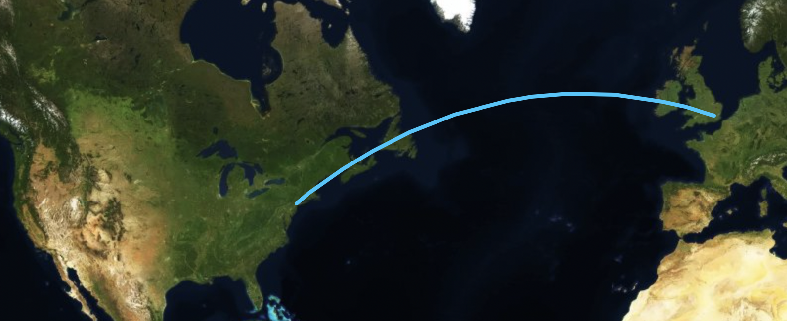
Houston to New York
The distance between the following two points \(([\phi_1,\lambda_1], [\phi_2,\lambda_2]) =([29.97, -95.35], [40.77, -73.98])\) (deg) is:
| Algorithm |
Procedure |
Result (meters) |
| Law of Cosines |
gcdist |
2272779.3057236285 |
| Haversine |
gcdist_haversine |
2272779.3057236294 |
| Vincenty |
gcdist_vincenty |
2272779.3057236290 |
Antipodal points
The distance between the following two antipodal points \(([\phi_1,\lambda_1], [\phi_2,\lambda_2]) = ([0, 0], [0.0, \pi/2])\) (radians) is:
| Algorithm |
Procedure |
Result (meters) |
| Law of Cosines |
gcdist |
20037508.342789244 |
| Haversine |
gcdist_haversine |
20037508.342789244 |
| Vincenty |
gcdist_vincenty |
20037508.342789244 |
Nearly antipodal points
The distance between the following two nearly antipodal points \(([\phi_1,\lambda_1], [\phi_2,\lambda_2]) = ([10^{-8}, 10^{-8}], [0.0, \pi/2])\) (radians) is:
| Algorithm |
Procedure |
Result (meters) |
| Law of Cosines |
gcdist |
20037508.342789244 |
| Haversine |
gcdist_haversine |
20037508.342789244 |
| Vincenty |
gcdist_vincenty |
20037508.252588764 |
Other methods
For a more accurate result, using an oblate-spheroid model of the Earth, the Vincenty inverse geodetic algorithm can be used (the equation above is just a special case of the more general algorithm when the ellipsoidal major and minor axes are equal). For the Houston to New York case, the difference between the spherical and oblate-spheroid equations is 282 meters.
See also

*Thaddeus Vincenty (1920--2002) Image source: [IAG Newsletter](http://www.gfy.ku.dk/~iag/newslett/news7606.htm)*
There are two standard problems in geodesy:
- Direct geodetic problem -- Given a point on the Earth (latitude and longitude) and the direction (azimuth) and distance from that point to a second point, determine the latitude and longitude of that second point.
- Inverse geodetic problem -- Given two points on the Earth, determine the azimuth and distance between them.
Assuming the Earth is an oblate spheroid, both of these can be solved using the iterative algorithms by Thaddeus Vincenty [1]. Modern Fortran versions of Vincenty's algorithms can be found in the geodesy module of the Fortran Astrodynamics Toolkit [2].
The direct algorithm was listed in an earlier post. If we assume a WGS84 Earth ellipsoid (a=6378.137 km, f=1/298.257223563), an example direct calculation is:
$$
\begin{array}{rcll}
\phi_1 &= & 29.97^{\circ} & \mathrm{(Latitude ~of ~ first ~ point)}\\
\lambda_1 &= & -95.35^{\circ} & \mathrm{(Longitude ~of ~ first ~point)} \\
Az &= & 20^{\circ} & \mathrm{(Azimuth)}\\
s &= & 50~\mathrm{km} & \mathrm{(Distance)}
\end{array}
$$
The latitude and longitude of the second point is:
$$
\begin{array}{rcl}
\phi_2 &= & 30.393716^{\circ} \\
\lambda_2 &= & -95.172057^{\circ} \\
\end{array}
$$
The more complicated inverse algorithm is listed here (based on the USNGS code from [1]):
subroutine inverse(a, rf, b1, l1, b2, l2, faz, baz, s, it, sig, lam, kind)

    use, intrinsic :: iso_fortran_env, wp => real64

    implicit none

    real(wp), intent(in) :: a !! Equatorial semimajor axis
    real(wp), intent(in) :: rf !! reciprocal flattening (1/f)
    real(wp), intent(in) :: b1 !! latitude of point 1 (rad, positive north)
    real(wp), intent(in) :: l1 !! longitude of point 1 (rad, positive east)
    real(wp), intent(in) :: b2 !! latitude of point 2 (rad, positive north)
    real(wp), intent(in) :: l2 !! longitude of point 2 (rad, positive east)
    real(wp), intent(out) :: faz !! Forward azimuth (rad, clockwise from north)
    real(wp), intent(out) :: baz !! Back azimuth (rad, clockwise from north)
    real(wp), intent(out) :: s !! Ellipsoidal distance
    integer, intent(out) :: it !! iteration count
    real(wp), intent(out) :: sig !! spherical distance on auxiliary sphere
    real(wp), intent(out) :: lam !! longitude difference on auxiliary sphere
    integer, intent(out) :: kind !! solution flag: kind=1, long-line; kind=2, antipodal

    real(wp) :: beta1, beta2, biga, bigb, bige, bigf, boa, &
                c, cosal2, coslam, cossig, costm, costm2, &
                cosu1, cosu2, d, dsig, ep2, l, prev, sinal, &
                sinlam, sinsig, sinu1, sinu2, tem1, tem2, &
                temp, test, z

    real(wp), parameter :: pi = acos(-1.0_wp)
    real(wp), parameter :: two_pi = 2.0_wp*pi
    real(wp), parameter :: tol = 1.0e-14_wp !! convergence tolerance
    real(wp), parameter :: eps = 1.0e-15_wp !! tolerance for zero

    boa = 1.0_wp - 1.0_wp/rf

    beta1 = atan(boa*tan(b1))
    sinu1 = sin(beta1)
    cosu1 = cos(beta1)
    beta2 = atan(boa*tan(b2))
    sinu2 = sin(beta2)
    cosu2 = cos(beta2)

    l = l2 - l1
    if (l > pi) l = l - two_pi
    if (l < -pi) l = l + two_pi
    prev = l
    test = l
    it = 0
    kind = 1
    lam = l

    longline: do ! long-line loop (kind=1)

        sinlam = sin(lam)
        coslam = cos(lam)
        temp = cosu1*sinu2 - sinu1*cosu2*coslam
        sinsig = sqrt((cosu2*sinlam)**2 + temp**2)
        cossig = sinu1*sinu2 + cosu1*cosu2*coslam
        sig = atan2(sinsig, cossig)
        if (abs(sinsig) < eps) then
            sinal = cosu1*cosu2*sinlam/sign(eps, sinsig)
        else
            sinal = cosu1*cosu2*sinlam/sinsig
        end if
        cosal2 = -sinal**2 + 1.0_wp
        if (abs(cosal2) < eps) then
            costm = -2.0_wp*(sinu1*sinu2/sign(eps, &
                                              cosal2)) + cossig
        else
            costm = -2.0_wp*(sinu1*sinu2/cosal2) + &
                    cossig
        end if
        costm2 = costm*costm
        c = ((-3.0_wp*cosal2 + 4.0_wp)/rf + 4.0_wp)* &
            cosal2/rf/16.0_wp

        antipodal: do ! antipodal loop (kind=2)

            it = it + 1
            d = (((2.0_wp*costm2 - 1.0_wp)*cossig*c + &
                  costm)*sinsig*c + sig)*(1.0_wp - c)/rf
            if (kind == 1) then
                lam = l + d*sinal
                if (abs(lam - test) >= tol) then
                    if (abs(lam) > pi) then
                        kind = 2
                        lam = pi
                        if (l < 0.0_wp) lam = -lam
                        sinal = 0.0_wp
                        cosal2 = 1.0_wp
                        test = 2.0_wp
                        prev = test
                        sig = pi - abs(atan(sinu1/cosu1) + &
                                    atan(sinu2/cosu2))
                        sinsig = sin(sig)
                        cossig = cos(sig)
                        c = ((-3.0_wp*cosal2 + 4.0_wp)/rf + &
                            4.0_wp)*cosal2/rf/16.0_wp
                        if (abs(sinal - prev) < tol) exit longline
                        if (abs(cosal2) < eps) then
                            costm = -2.0_wp*(sinu1*sinu2/ &
                                            sign(eps, cosal2)) + cossig
                        else
                            costm = -2.0_wp*(sinu1*sinu2/cosal2) + &
                                    cossig
                        end if
                        costm2 = costm*costm
                        cycle antipodal
                    end if
                    if (((lam - test)*(test - prev)) < 0.0_wp .and. it > 5) &
                        lam = (2.0_wp*lam + 3.0_wp*test + prev)/6.0_wp
                    prev = test
                    test = lam
                    cycle longline
                end if
            else
                sinal = (lam - l)/d
                if (((sinal - test)*(test - prev)) < 0.0_wp .and. it > 5) &
                    sinal = (2.0_wp*sinal + 3.0_wp*test + prev)/6.0_wp
                prev = test
                test = sinal
                cosal2 = -sinal**2 + 1.0_wp
                sinlam = sinal*sinsig/(cosu1*cosu2)
                coslam = -sqrt(abs(-sinlam**2 + 1.0_wp))
                lam = atan2(sinlam, coslam)
                temp = cosu1*sinu2 - sinu1*cosu2*coslam
                sinsig = sqrt((cosu2*sinlam)**2 + temp**2)
                cossig = sinu1*sinu2 + cosu1*cosu2*coslam
                sig = atan2(sinsig, cossig)
                c = ((-3.0_wp*cosal2 + 4.0_wp)/rf + 4.0_wp)* &
                    cosal2/rf/16.0_wp
                if (abs(sinal - prev) >= tol) then
                if (abs(cosal2) < eps) then
                    costm = -2.0_wp*(sinu1*sinu2/ &
                                     sign(eps, cosal2)) + cossig
                else
                    costm = -2.0_wp*(sinu1*sinu2/cosal2) + &
                            cossig
                end if
                costm2 = costm*costm
                cycle antipodal
                end if
            end if

            exit longline

        end do antipodal

    end do longline

    if (kind == 2) then ! antipodal
        faz = sinal/cosu1
        baz = sqrt(-faz**2 + 1.0_wp)
        if (temp < 0.0_wp) baz = -baz
        faz = atan2(faz, baz)
        tem1 = -sinal
        tem2 = sinu1*sinsig - cosu1*cossig*baz
        baz = atan2(tem1, tem2)
    else ! long-line
        tem1 = cosu2*sinlam
        tem2 = cosu1*sinu2 - sinu1*cosu2*coslam
        faz = atan2(tem1, tem2)
        tem1 = -cosu1*sinlam
        tem2 = sinu1*cosu2 - cosu1*sinu2*coslam
        baz = atan2(tem1, tem2)
    end if

    if (faz < 0.0_wp) faz = faz + two_pi
    if (baz < 0.0_wp) baz = baz + two_pi
    ep2 = 1.0_wp/(boa*boa) - 1.0_wp
    bige = sqrt(1.0_wp + ep2*cosal2)
    bigf = (bige - 1.0_wp)/(bige + 1.0_wp)
    biga = (1.0_wp + bigf*bigf/4.0_wp)/(1.0_wp - bigf)
    bigb = bigf*(1.0_wp - 0.375_wp*bigf*bigf)
    z = bigb/6.0_wp*costm*(-3.0_wp + 4.0_wp* &
                           sinsig**2)*(-3.0_wp + 4.0_wp*costm2)
    dsig = bigb*sinsig*(costm + bigb/4.0_wp* &
                        (cossig*(-1.0_wp + 2.0_wp*costm2) - z))
    s = (boa*a)*biga*(sig - dsig)

end subroutine inverse
For the same ellipsoid, an example inverse calculation is:
$$
\begin{array}{rcll}
\phi_1 &= & 29.97^{\circ} & \mathrm{(Latitude ~of ~ first ~ point)}\\
\lambda_1 &= & -95.35^{\circ} & \mathrm{(Longitude ~of ~ first ~point)} \\
\phi_2 &= & 40.77^{\circ} & \mathrm{(Latitude ~of ~ second ~ point)}\\
\lambda_2 &= & -73.98^{\circ} & \mathrm{(Longitude ~of ~ second ~point)}
\end{array}
$$
The azimuth and distance from the first to the second point is:
$$
\begin{array}{rcl}
Az &= & 52.400056^{\circ} & \mathrm{(Azimuth)}\\
s &= & 2272.497~\mathrm{km} & \mathrm{(Distance)}
\end{array}
$$
References

The IAU Working Group on Cartographic Coordinates and Rotational Elements (WGCCRE) is the keeper of official models that describe the cartographic coordinates and rotational elements of planetary bodies (such as the Earth, satellites, minor planets, and comets). Periodically, they release a report containing the coefficients to compute body orientations, based on the latest data available. These coefficients allow one to compute the rotation matrix from the ICRF frame to a body-fixed frame (for example, IAU Earth) by giving the direction of the pole vector and the prime meridian location as functions of time. An example Fortran module illustrating this for the IAU Earth frame is given below. The coefficients are taken from the 2009 IAU report [Reference 1]. Note that the IAU models are also available in SPICE (as "IAU_EARTH", "IAU_MOON", etc.). For Earth, the IAU model is not suitable for use in applications that require the highest possible accuracy (for that a more complex model would be necessary), but is quite acceptable for many applications.
module iau_orientation_module

use, intrinsic :: iso_fortran_env, only: wp => real64

implicit none

private

!constants:
real(wp),parameter :: zero = 0.0_wp
real(wp),parameter :: one = 1.0_wp
real(wp),parameter :: pi = acos(-one)
real(wp),parameter :: pi2 = pi/2.0_wp
real(wp),parameter :: deg2rad = pi/180.0_wp
real(wp),parameter :: sec2day = one/86400.0_wp
real(wp),parameter :: sec2century = one/3155760000.0_wp

public :: icrf_to_iau_earth

contains

!Rotation matrix from ICRF to IAU_EARTH
pure function icrf_to_iau_earth(et) result(rotmat)

implicit none

real(wp),intent(in) :: et !ephemeris time [sec from J2000]
real(wp),dimension(3,3) :: rotmat !rotation matrix

real(wp) :: w,dec,ra,d,t
real(wp),dimension(3,3) :: tmp

d = et * sec2day !days from J2000
t = et * sec2century !Julian centuries from J2000

ra = ( - 0.641_wp * t ) * deg2rad
dec = ( 90.0_wp - 0.557_wp * t ) * deg2rad
w = ( 190.147_wp + 360.9856235_wp * d ) * deg2rad

!it is a 3-1-3 rotation:
tmp = matmul( rotmat_x(pi2-dec), rotmat_z(pi2+ra) )
rotmat = matmul( rotmat_z(w), tmp )

end function icrf_to_iau_earth

!The 3x3 rotation matrix for a rotation about the x-axis.
pure function rotmat_x(angle) result(rotmat)

implicit none

real(wp),dimension(3,3) :: rotmat !rotation matrix
real(wp),intent(in) :: angle !angle [rad]

real(wp) :: c,s

c = cos(angle)
s = sin(angle)

rotmat = reshape([one, zero, zero, &
                  zero, c, -s, &
                  zero, s, c],[3,3])

end function rotmat_x

!The 3x3 rotation matrix for a rotation about the z-axis.
pure function rotmat_z(angle) result(rotmat)

implicit none

real(wp),dimension(3,3) :: rotmat !rotation matrix
real(wp),intent(in) :: angle !angle [rad]

real(wp) :: c,s

c = cos(angle)
s = sin(angle)

rotmat = reshape([ c, -s, zero, &
                   s, c, zero, &
                   zero, zero, one ],[3,3])

end function rotmat_z

end module iau_orientation_module
References
- B. A. Archinal, et al., "Report of the IAU Working Group on Cartographic Coordinates and Rotational Elements: 2009", Celest Mech Dyn Astr (2011) 109:101-135.
- J. Williams, Fortran Astrodynamics Toolkit - iau_orientation_module [GitHub]
The gravitational potential of a non-homogeneous celestial body at radius \(r\), latitude \(\phi\) , and longitude \(\lambda\) can be represented in spherical coordinates as:
$$
U = \frac{\mu}{r} [ 1 + \sum\limits_{n=2}^{n_{max}} \sum\limits_{m=0}^{n} \left( \frac{r_e}{r} \right)^n P_{n,m}(\sin \phi) ( C_{n,m} \cos m\lambda + S_{n,m} \sin m\lambda ) ]
$$
Where \(r_e\) is the radius of the body, \(\mu\) is the gravitational parameter of the body, \(C_{n,m}\) and \(S_{n,m}\) are spherical harmonic coefficients, \(P_{n,m}\) are Associated Legendre Functions, and \(n_{max}\) is the desired degree and order of the approximation. The acceleration of a spacecraft at this location is the gradient of this potential. However, if the conventional representation of the potential given above is used, it will result in singularities at the poles \((\phi = \pm 90^{\circ})\), since the longitude becomes undefined at these points. (Also, evaluation on a computer would be relatively slow due to the number of sine and cosine terms).
A geopotential formulation that eliminates the polar singularity was devised by Samuel Pines in the early 1970s [1]. Over the years, various implementations and refinements of this algorithm and other similar algorithms have been published [2-7], mostly at the Johnson Space Center. The Fortran 77 code in Mueller [2] and Lear [4-5] is easily translated into modern Fortran. The Pines algorithm code from Spencer [3] appears to contain a few bugs, so translation is more of a challenge. A modern Fortran version (with bugs fixed) is presented below:
subroutine gravpot(r,nmax,re,mu,c,s,acc)

use, intrinsic :: iso_fortran_env, only: wp => real64

implicit none

real(wp),dimension(3),intent(in) :: r !position vector
integer,intent(in) :: nmax !degree/order
real(wp),intent(in) :: re !body radius
real(wp),intent(in) :: mu !grav constant
real(wp),dimension(nmax,0:nmax),intent(in) :: c !coefficients
real(wp),dimension(nmax,0:nmax),intent(in) :: s !
real(wp),dimension(3),intent(out) :: acc !grav acceleration

!local variables:
real(wp),dimension(nmax+1) :: creal, cimag, rho
real(wp),dimension(nmax+1,nmax+1) :: a,d,e,f
integer :: nax0,i,j,k,l,n,m
real(wp) :: rinv,ess,t,u,r0,rhozero,a1,a2,a3,a4,fac1,fac2,fac3,fac4
real(wp) :: ci1,si1

real(wp),parameter :: zero = 0.0_wp
real(wp),parameter :: one = 1.0_wp

!JW : not done in original paper,
!     but seems to be necessary
!     (probably assumed the compiler
!      did it automatically)
a = zero
d = zero
e = zero
f = zero

!get the direction cosines ess, t and u:

nax0 = nmax + 1
rinv = one/norm2(r)
ess  = r(1) * rinv
t    = r(2) * rinv
u    = r(3) * rinv

!generate the functions creal, cimag, a, d, e, f and rho:

r0       = re*rinv
rhozero  = mu*rinv    !JW: typo in original paper
rho(1)   = r0*rhozero
creal(1) = ess
cimag(1) = t
d(1,1)   = zero
e(1,1)   = zero
f(1,1)   = zero
a(1,1)   = one

do i=2,nax0

    if (i/=nax0) then !JW : to prevent access
        ci1 = c(i,1)  !     to c,s outside bounds
        si1 = s(i,1)
    else
        ci1 = zero
        si1 = zero
    end if

    rho(i)   = r0*rho(i-1)
    creal(i) = ess*creal(i-1) - t*cimag(i-1)
    cimag(i) = ess*cimag(i-1) + t*creal(i-1)
    d(i,1)   = ess*ci1 + t*si1
    e(i,1)   = ci1
    f(i,1)   = si1
    a(i,i)   = (2*i-1)*a(i-1,i-1)
    a(i,i-1) = u*a(i,i)

    do k=2,i

        if (i/=nax0) then
            d(i,k) = c(i,k)*creal(k)   + s(i,k)*cimag(k)
            e(i,k) = c(i,k)*creal(k-1) + s(i,k)*cimag(k-1)
            f(i,k) = s(i,k)*creal(k-1) - c(i,k)*cimag(k-1)
        end if

        !JW : typo here in original paper
        ! (should be GOTO 1, not GOTO 10)
        if (i/=2) then
            L = i-2
            do j=1,L
                a(i,i-j-1) = (u*a(i,i-j)-a(i-1,i-j))/(j+1)
            end do
        end if

    end do

end do

!compute auxiliary quantities a1, a2, a3, a4

a1 = zero
a2 = zero
a3 = zero
a4 = rhozero*rinv

do n=2,nmax

    fac1 = zero
    fac2 = zero
    fac3 = a(n,1)  *c(n,0)
    fac4 = a(n+1,1)*c(n,0)

    do m=1,n
        fac1 = fac1 + m*a(n,m)    *e(n,m)
        fac2 = fac2 + m*a(n,m)    *f(n,m)
        fac3 = fac3 +   a(n,m+1)  *d(n,m)
        fac4 = fac4 +   a(n+1,m+1)*d(n,m)
    end do

    a1 = a1 + rinv*rho(n)*fac1
    a2 = a2 + rinv*rho(n)*fac2
    a3 = a3 + rinv*rho(n)*fac3
    a4 = a4 + rinv*rho(n)*fac4

end do

!gravitational acceleration vector:

acc(1) = a1 - ess*a4
acc(2) = a2 - t*a4
acc(3) = a3 - u*a4

end subroutine gravpot
References
- S. Pines. "Uniform Representation of the Gravitational Potential and its Derivatives", AIAA Journal, Vol. 11, No. 11, (1973), pp. 1508-1511.
- A. C. Mueller, "A Fast Recursive Algorithm for Calculating the Forces due to the Geopotential (Program: GEOPOT)", JSC Internal Note 75-FM-42, June 9, 1975.
- J. L. Spencer, "Pines Nonsingular Gravitational Potential Derivation, Description and Implementation", NASA Contractor Report 147478, February 9, 1976.
- W. M. Lear, "The Gravitational Acceleration Equations", JSC Internal Note 86-FM-15, April 1986.
- W. M. Lear, "The Programs TRAJ1 and TRAJ2", JSC Internal Note 87-FM-4, April 1987.
- R. G. Gottlieb, "Fast Gravity, Gravity Partials, Normalized Gravity, Gravity Gradient Torque and Magnetic Field: Derivation, Code and Data", NASA Contractor Report 188243, February, 1993.
- R. A. Eckman, A. J. Brown, and D. R. Adamo, "Normalization of Gravitational Acceleration Models", JSC-CN-23097, January 24, 2011.
The "direct" geodetic problem is: given the latitude and longitude of one point and the azimuth and distance to a second point, determine the latitude and longitude of that second point. The solution can be obtained using the algorithm by Polish American geodesist Thaddeus Vincenty [1]. A modern Fortran implementation is given below:
subroutine direct(a,f,glat1,glon1,glat2,glon2,faz,baz,s)

use, intrinsic :: iso_fortran_env, wp => real64

implicit none

real(wp),intent(in) :: a !semimajor axis of ellipsoid [m]
real(wp),intent(in) :: f !flattening of ellipsoid [-]
real(wp),intent(in) :: glat1 !latitude of 1 [rad]
real(wp),intent(in) :: glon1 !longitude of 1 [rad]
real(wp),intent(in) :: faz !forward azimuth 1->2 [rad]
real(wp),intent(in) :: s !distance from 1->2 [m]
real(wp),intent(out) :: glat2 !latitude of 2 [rad]
real(wp),intent(out) :: glon2 !longitude of 2 [rad]
real(wp),intent(out) :: baz !back azimuth 2->1 [rad]

real(wp) :: r,tu,sf,cf,cu,su,sa,csa,c2a,x,c,d,y,sy,cy,cz,e

real(wp),parameter :: pi = acos(-1.0_wp)
real(wp),parameter :: eps = 0.5e-13_wp

r = 1.0_wp-f
tu = r*sin(glat1)/cos(glat1)
sf = sin(faz)
cf = cos(faz)
baz = 0.0_wp
if (cf/=0.0_wp) baz = atan2(tu,cf)*2.0_wp
cu = 1.0_wp/sqrt(tu*tu+1.0_wp)
su = tu*cu
sa = cu*sf
c2a = -sa*sa+1.0_wp
x = sqrt((1.0_wp/r/r-1.0_wp)*c2a+1.0_wp)+1.0_wp
x = (x-2.0_wp)/x
c = 1.0_wp-x
c = (x*x/4.0_wp+1.0_wp)/c
d = (0.375_wp*x*x-1.0_wp)*x
tu = s/r/a/c
y = tu
do
    sy = sin(y)
    cy = cos(y)
    cz = cos(baz+y)
    e = cz*cz*2.0_wp-1.0_wp
    c = y
    x = e*cy
    y = e+e-1.0_wp
    y = (((sy*sy*4.0_wp-3.0_wp)*y*cz*d/6.0_wp+x)*d/4.0_wp-cz)*sy*d+tu
    if (abs(y-c)<=eps) exit
end do
baz = cu*cy*cf-su*sy
c = r*sqrt(sa*sa+baz*baz)
d = su*cy+cu*sy*cf
glat2 = atan2(d,c)
c = cu*cy-su*sy*cf
x = atan2(sy*sf,c)
c = ((-3.0_wp*c2a+4.0_wp)*f+4.0_wp)*c2a*f/16.0_wp
d = ((e*cy*c+cz)*sy*c+y)*sa
glon2 = glon1+x-(1.0_wp-c)*d*f
baz = atan2(sa,baz)+pi

end subroutine direct
References
- T. Vincenty, "Direct and Inverse Solutions of Geodesics on the Ellipsoid with Application of Nested Equations", Survey Review XXII. 176, April 1975. [sourcecode from the U.S. National Geodetic Survey].
For many years, I have used the closed-form solution from Heikkinen [1] for converting Cartesian coordinates to geodetic latitude and altitude. I've never actually seen the original reference (which is in German). I coded up the algorithm from the table given in [2], and have used it ever since, in school and also at work. At one point I compared it with various other closed-form algorithms, and never found one that was faster and still had the same level of accuracy. However, I recently happened to stumble upon Olson's method [3], which seems to be better.
A Fortran implementation of Olson's algorithm is:
pure subroutine olson(rvec, a, b, h, lon, lat)

    use, intrinsic :: iso_fortran_env, wp=>real64 !double precision

    implicit none

    real(wp),dimension(3),intent(in) :: rvec !position vector [km]
    real(wp),intent(in)  :: a   ! geoid semimajor axis [km]
    real(wp),intent(in)  :: b   ! geoid semiminor axis [km]
    real(wp),intent(out) :: h   ! geodetic altitude [km]
    real(wp),intent(out) :: lon ! longitude [rad]
    real(wp),intent(out) :: lat ! geodetic latitude [rad]

    real(wp) :: f,x,y,z,e2,a1,a2,a3,a4,a5,a6,w,zp,&
                w2,r2,r,s2,c2,u,v,s,ss,c,g,rg,rf,m,p,z2

    x = rvec(1)
    y = rvec(2)
    z = rvec(3)
    f = (a-b)/a
    e2 = f * (2.0_wp - f)
    a1 = a * e2
    a2 = a1 * a1
    a3 = a1 * e2 / 2.0_wp
    a4 = 2.5_wp * a2
    a5 = a1 + a3
    a6 = 1.0_wp - e2
    zp = abs(z)
    w2 = x*x + y*y
    w = sqrt(w2)
    z2 = z * z
    r2 = z2 + w2
    r = sqrt(r2)

    if (r < 100.0_wp) then

        lat = 0.0_wp
        lon = 0.0_wp
        h = -1.0e7_wp

    else

        s2 = z2 / r2
        c2 = w2 / r2
        u = a2 / r
        v = a3 - a4 / r

        if (c2 > 0.3_wp) then
            s = (zp / r) * (1.0_wp + c2 * (a1 + u + s2 * v) / r)
            lat = asin(s)
            ss = s * s
            c = sqrt(1.0_wp - ss)
        else
            c = (w / r) * (1.0_wp - s2 * (a5 - u - c2 * v) / r)
            lat = acos(c)
            ss = 1.0_wp - c * c
            s = sqrt(ss)
        end if

        g = 1.0_wp - e2 * ss
        rg = a / sqrt(g)
        rf = a6 * rg
        u = w - rg * c
        v = zp - rf * s
        f = c * u + s * v
        m = c * v - s * u
        p = m / (rf / g + f)
        lat = lat + p
        if (z < 0.0_wp) lat = -lat
        h = f + m * p / 2.0_wp
        lon = atan2( y, x )

    end if

end subroutine olson
For comparison, Heikkinen's algorithm is:
pure subroutine heikkinen(rvec, a, b, h, lon, lat)

    use, intrinsic :: iso_fortran_env, wp=>real64 !double precision

    implicit none

    real(wp),dimension(3),intent(in) :: rvec !position vector [km]
    real(wp),intent(in)  :: a    ! geoid semimajor axis [km]
    real(wp),intent(in)  :: b    ! geoid semiminor axis [km]
    real(wp),intent(out) :: h    ! geodetic altitude [km]
    real(wp),intent(out) :: lon  ! longitude [rad]
    real(wp),intent(out) :: lat  ! geodetic latitude [rad]

    real(wp) :: f,e_2,ep,r,e2,ff,g,c,s,pp,q,r0,u,v,z0,x,y,z,z2,r2,tmp,a2,b2

    x = rvec(1)
    y = rvec(2)
    z = rvec(3)
    a2 = a*a
    b2 = b*b
    f = (a-b)/a
    e_2 = (2.0_wp*f-f*f)
    ep = sqrt(a2/b2 - 1.0_wp)
    z2 = z*z
    r = sqrt(x**2 + y**2)
    r2 = r*r
    e2 = a2 - b2
    ff = 54.0_wp * b2 * z2
    g = r2 + (1.0_wp - e_2)*z2 - e_2*e2
    c = e_2**2 * ff * r2 / g**3
    s = (1.0_wp + c + sqrt(c**2 + 2.0_wp*c))**(1.0_wp/3.0_wp)
    pp = ff / ( 3.0_wp*(s + 1.0_wp/s + 1.0_wp)**2 * g**2 )
    q = sqrt( 1.0_wp + 2.0_wp*e_2**2 * pp )
    r0 = -pp*e_2*r/(1.0_wp+q) + &
        sqrt( max(0.0_wp, 1.0_wp/2.0_wp * a2 * (1.0_wp + 1.0_wp/q) - &
        ( pp*(1.0_wp-e_2)*z2 )/(q*(1.0_wp+q)) - &
        1.0_wp/2.0_wp * pp * r2) )
    u = sqrt( (r - e_2*r0)**2 + z2 )
    v = sqrt( (r - e_2*r0)**2 + (1.0_wp - e_2)*z2 )
    z0 = b**2 * z / (a*v)
    h = u*(1.0_wp - b2/(a*v) )
    lat = atan2( (z + ep**2*z0), r )
    lon = atan2( y, x )

end subroutine heikkinen
Olson's is about 1.5 times faster on my 2.53 GHz i5 laptop, when both are compiled using gfortran with -O2 optimization (Olson: 3,743,212 cases/sec, Heikkinen: 2,499,670 cases/sec). The level of accuracy is about the same for each method.
References
- M. Heikkinen, "Geschlossene formeln zur berechnung raumlicher geodatischer koordinaten aus rechtwinkligen Koordinaten". Z. Ermess., 107 (1982), 207-211 (in German).
- E. D. Kaplan, "Understanding GPS: Principles and Applications", Artech House, 1996.
- D. K. Olson, "Converting Earth-Centered, Earth-Fixed Coordinates to Geodetic Coordinates," IEEE Transactions on Aerospace and Electronic Systems, 32 (1996) 473-476.