Nov 11, 2021
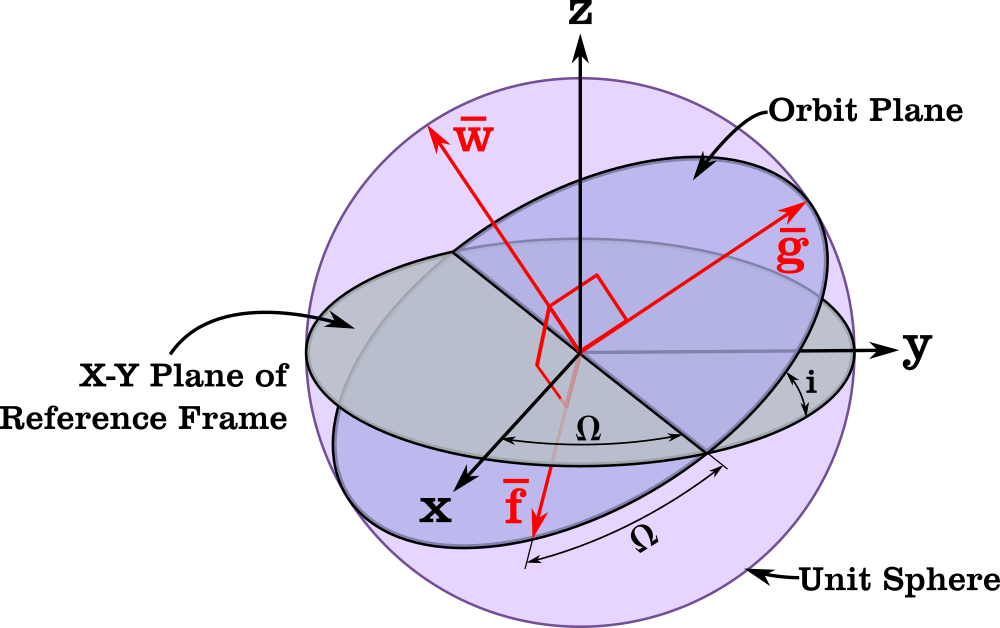
The Orbital Coordinate Frame used for Equinoctial Elements (see Reference [5])
Last time, I mentioned an alternative orbital element set different from the classical elements.
Modified equinoctial elements \((p,f,g,h,k,L)\) are another alternative that are applicable to all orbits and have nonsingular equations of motion (except for a singularity at \(i = \pi\)). They are defined as [1]:
- \(p = a (1 - e^2)\)
- \(f = e \cos (\omega + \Omega)\)
- \(g = e \sin (\omega + \Omega)\)
- \(h = \tan (i/2) \cos \Omega\)
- \(k = \tan (i/2) \sin \Omega\)
- \(L = \Omega + \omega + \nu\)
Where \(a\) is the semimajor axis, \(p\) is the semi-latus rectum, \(i\) is the inclination, \(e\) is the eccentricity, \(\omega\) is the argument of periapsis, \(\Omega\) is the right ascension of the ascending node, \(L\) is the true longitude, and \(\nu\) is the true anomaly. \((f,g)\) are the x and y components of the eccentricity vector in the orbital frame, and \((h,k)\) are the x and y components of the node vector in the orbital frame.
The conversion from Cartesian state (position and velocity) to modified equinoctial elements is given in this Fortran subroutine:
subroutine cartesian_to_equinoctial(mu,rv,evec)

use iso_fortran_env, only: wp => real64

implicit none

real(wp),intent(in)               :: mu    !! central body gravitational parameter (km^3/s^2)
real(wp),dimension(6),intent(in)  :: rv    !! Cartesian state vector
real(wp),dimension(6),intent(out) :: evec  !! Modified equinoctial element vector: [p,f,g,h,k,L]

real(wp),dimension(3) :: r,v,hvec,hhat,ecc,fhat,ghat,rhat,vhat
real(wp) :: hmag,rmag,p,f,g,h,k,L,kk,hh,s2,tkh,rdv

r = rv(1:3)
v = rv(4:6)

rdv      = dot_product(r,v)
rhat     = unit(r)
rmag     = norm2(r)
hvec     = cross(r,v)
hmag     = norm2(hvec)
hhat     = unit(hvec)
vhat     = (rmag*v - rdv*rhat)/hmag
p        = hmag*hmag / mu
k        = hhat(1)/(1.0_wp + hhat(3))
h        = -hhat(2)/(1.0_wp + hhat(3))
kk       = k*k
hh       = h*h
s2       = 1.0_wp+hh+kk
tkh      = 2.0_wp*k*h
ecc      = cross(v,hvec)/mu - rhat
fhat(1)  = 1.0_wp-kk+hh
fhat(2)  = tkh
fhat(3)  = -2.0_wp*k
ghat(1)  = tkh
ghat(2)  = 1.0_wp+kk-hh
ghat(3)  = 2.0_wp*h
fhat     = fhat/s2
ghat     = ghat/s2
f        = dot_product(ecc,fhat)
g        = dot_product(ecc,ghat)
L        = atan2(rhat(2)-vhat(1),rhat(1)+vhat(2))

evec = [p,f,g,h,k,L]

end subroutine cartesian_to_equinoctial
Where cross is a cross product function and unit is a unit vector function (\(\mathbf{u} = \mathbf{v} / |\mathbf{v}|\)).
The inverse routine (modified equinoctial to Cartesian) is:
subroutine equinoctial_to_cartesian(mu,evec,rv)

use iso_fortran_env, only: wp => real64

implicit none

real(wp),intent(in)               :: mu   !! central body gravitational parameter (km^3/s^2)
real(wp),dimension(6),intent(in)  :: evec !! Modified equinoctial element vector : [p,f,g,h,k,L]
real(wp),dimension(6),intent(out) :: rv   !! Cartesian state vector

real(wp) :: p,f,g,h,k,L,s2,r,w,cL,sL,smp,hh,kk,tkh
real(wp) :: x,y,xdot,ydot
real(wp),dimension(3) :: fhat,ghat

p = evec(1)
f = evec(2)
g = evec(3)
h = evec(4)
k = evec(5)
L = evec(6)

kk      = k*k
hh      = h*h
tkh     = 2.0_wp*k*h
s2      = 1.0_wp + hh + kk
cL      = cos(L)
sL      = sin(L)
w       = 1.0_wp + f*cL + g*sL
r       = p/w
smp     = sqrt(mu/p)
fhat(1) = 1.0_wp-kk+hh
fhat(2) = tkh
fhat(3) = -2.0_wp*k
ghat(1) = tkh
ghat(2) = 1.0_wp+kk-hh
ghat(3) = 2.0_wp*h
fhat    = fhat/s2
ghat    = ghat/s2
x       = r*cL
y       = r*sL
xdot    = -smp * (g + sL)
ydot    =  smp * (f + cL)

rv(1:3) = x*fhat + y*ghat
rv(4:6) = xdot*fhat + ydot*ghat

end subroutine equinoctial_to_cartesian
The equations of motion are:
subroutine modified_equinoctial_derivs(mu,evec,scn,evecd)

use iso_fortran_env, only: wp => real64

implicit none

real(wp),intent(in)               :: mu    !! central body gravitational parameter (km^3/s^2)
real(wp),dimension(6),intent(in)  :: evec  !! modified equinoctial element vector : [p,f,g,h,k,L]
real(wp),dimension(3),intent(in)  :: scn   !! Perturbation (in the RSW frame) (km/sec^2)
real(wp),dimension(6),intent(out) :: evecd !! derivative of `evec`

real(wp) :: p,f,g,h,k,L,c,s,n,sqrtpm,sl,cl,s2no2w,s2,w

p      = evec(1)
f      = evec(2)
g      = evec(3)
h      = evec(4)
k      = evec(5)
L      = evec(6)
s      = scn(1)
c      = scn(2)
n      = scn(3)
sqrtpm = sqrt(p/mu)
sl     = sin(L)
cl     = cos(L)
s2     = 1.0_wp + h*h + k*k
w      = 1.0_wp + f*cl + g*sl
s2no2w = s2*n / (2.0_wp*w)

evecd(1) = (2.0_wp*p*c/w) * sqrtpm
evecd(2) = sqrtpm * ( s*sl + ((w+1.0_wp)*cl+f)*c/w - g*n*(h*sl-k*cl)/w )
evecd(3) = sqrtpm * (-s*cl + ((w+1.0_wp)*sl+g)*c/w + f*n*(h*sl-k*cl)/w )
evecd(4) = sqrtpm * s2no2w * cl
evecd(5) = sqrtpm * s2no2w * sl
evecd(6) = sqrt(mu*p)*(w/p)**2 + sqrtpm * ((h*sl-k*cl)*n)/w

end subroutine modified_equinoctial_derivs
The 3-element scn vector contains the components of the perturbing acceleration (e.g. from a thrusting engine, other celestial bodies, etc.) in the directions perpendicular to the radius vector, in the "along track" direction, and the direction of the angular momentum vector.
Integration using modified equinoctial elements will generally be more efficient than a Cowell type integration of the Cartesian state elements. You only have to worry about the one singularity (note that there is also an alternate retrograde formulation where the singularity is moved to \(i = 0\)).
See also
References
- M. J. H. Walker, B. Ireland, Joyce Owens, "A Set of Modified Equinoctial Orbit Elements" Celestial Mechanics, Volume 36, Issue 4, p 409-419. (1985)
- Walker, M. J. H, "Erratum - a Set of Modified Equinoctial Orbit Elements" Celestial Mechanics, Volume 38, Issue 4, p 391-392. (1986)
- Broucke, R. A. & Cefola, P. J., "On the Equinoctial Orbit Elements" Celestial Mechanics, Volume 5, Issue 3, p 303-310. (1972)
- D. A. Danielson, C. P. Sagovac, B. Neta, L. W. Early, "Semianalytic Satellite Theory", Naval Postgraduate School Department of Mathematics, 1995
- P. J. Cefola, "Equinoctial orbit elements - Application to artificial satellite orbits", Astrodynamics Conference, 11-12 September 1972.
Oct 25, 2021
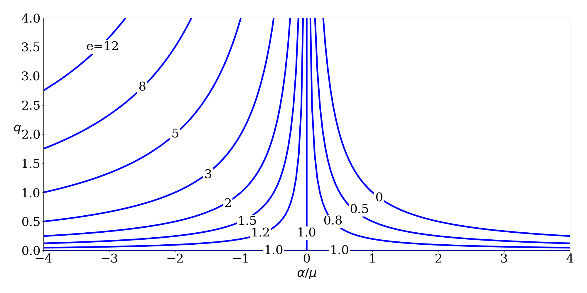
Variation of $q$ with $\alpha/\mu ~(=1/a)$ for selected values of $e$. (see Reference [1])
There are various different 6-element sets that can be used to represent the state (position and velocity) of a spacecraft. The classical Keplerian element set (\(a\), \(e\), \(i\), \(\Omega\), \(\omega\), \(\nu\)) is perhaps the most common, but not the only one. The Gooding universal element set [1] is:
- \(\alpha\) : twice the negative energy per unit mass (\(2 \mu / r - v^2\) or \(\mu/a\))
- \(q\) : periapsis radius magnitude (a.k.a. \(r_p\))
- \(i\) : inclination
- \(\Omega\) : right ascension of the ascending node
- \(\omega\) : argument of periapsis
- \(\tau\) : time since last periapsis passage
The nice thing about this set is that it is always defined, even for parabolas and rectilinear orbits (which other orbital element sets tend to ignore). A table from [1] shows the relationship between \(\alpha\) and \(q\) for the different types of conics:
|
\(\alpha > 0\) |
\(\alpha = 0\) |
\(\alpha < 0\) |
| \(q > 0\) |
general ellipse |
general parabola |
general hyperbola |
| \(q = 0\) |
rectilinear ellipse |
rectilinear parabola |
rectilinear hyperbola |
One advantage of this formulation is for trajectory optimization purposes, since if \(\alpha\) is an optimization variable, the orbit can transition from an ellipse to a hyperbola while iterating without encountering any singularities (which is not true if semimajor axis and eccentricity are being used, since \(a \rightarrow \infty\) for a parabola and then becomes negative for a hyperbola).
Gooding's original paper from 1988 includes Fortran 77 code for the transformations to and from position and velocity, coded with great care to avoid loss of accuracy due to numerical issues. Two other papers [2-3] also include some components of the algorithm. Modernized versions of these routines can be found in the Fortran Astrodynamics Toolkit. For example, a modernized version of ekepl1 (from [2]) for solving Kepler's equation:
pure function ekepl1(em, e)
  !!  Solve kepler's equation, `em = ekepl - e*sin(ekepl)`,
  !!  with legendre-based starter and halley iterator

  implicit none

  real(wp) :: ekepl1
  real(wp),intent(in) :: em
  real(wp),intent(in) :: e

  real(wp) :: c,s,psi,xi,eta,fd,fdd,f

  real(wp),parameter :: testsq = 1.0e-8_wp

  c = e*cos(em)
  s = e*sin(em)
  psi = s/sqrt(1.0_wp - c - c + e*e)

  do
    xi = cos(psi)
    eta = sin(psi)
    fd = (1.0_wp - c*xi) + s*eta
    fdd = c*eta + s*xi
    f = psi - fdd
    psi = psi - f*fd/(fd*fd - 0.5_wp*f*fdd)
    if (f*f < testsq) exit
   end do

   ekepl1 = em + psi

end function ekepl1
The Gooding universal element set can be found in NASA's Copernicus tool, and is being used in the design and optimization of the Artemis I trajectory.
See also
References
- R. H. Gooding, "On universal elements, and conversion procedures to and from position and velocity" Celestial Mechanics 44 (1988), 283-298.
- A. W. Odell, R. H. Gooding, "Procedures for solving Kepler's equation" Celestial Mechanics 38 (1986), 307-334.
- R. H. Gooding, A. W. Odell. "The hyperbolic Kepler equation (and the elliptic equation revisited)" Celestial Mechanics 44 (1988), 267-282.
- J, Williams, J. S. Senent, and D. E. Lee, "Recent improvements to the copernicus trajectory design and optimization system", Advances in the Astronautical Sciences 143, January 2012 (AAS 12-236)
- G. Hintz, "Survey of Orbit Element Sets", Journal of Guidance Control and Dynamics, 31(3):785-790, May 2008
Oct 24, 2021

The drag force magnitude on a spacecraft can be computed using the following equation:
$$ d = \frac{1}{2} \rho v^2 A C_D$$
Which can be easily implemented in the following Fortran function:
pure function drag(density, v, area, cd)

    use iso_fortran_env, only: wp => real64

    implicit none

    real(wp) :: drag !! drag force magnitude (N)
    real(wp), intent(in) :: density !! atmospheric density (kg/m^3)
    real(wp), intent(in) :: v       !! relative velocity magnitude (m/s)
    real(wp), intent(in) :: area    !! spacecraft cross-sectional area (m^2)
    real(wp), intent(in) :: cd      !! spacecraft drag coefficient

    drag = 0.5_wp * density * v**2 * area * cd

end function drag
The density \(\rho\) is computed using an atmosphere model. Here is a listing of some atmosphere model codes available in Fortran:
See also
- Fox & Mcdonald, "Introduction To Fluid Mechanics", Wiley
- Drag Coefficient [Wikipedia]
- U.S. Standard Atmosphere, 1976, U.S. Government Printing Office, Washington, D.C., 1976.
- ModelWeb Catalogue and Archive [NASA GSFC]
- W. W. Vaughan, "Guide to Reference and Standard Atmospheric Models", AIAA G-003C-2010, January 2010
Oct 18, 2021
If we assume that the Earth is a sphere of radius \(r\), the shortest distance between two sites (\([\phi_1,\lambda_1]\) and \([\phi_2,\lambda_2]\)) on the surface is the great-circle distance, which can be computed in several ways:
Law of Cosines equation:
$$
d = r \arccos\bigl(\sin\phi_1\cdot\sin\phi_2+\cos\phi_1\cdot\cos\phi_2\cdot\cos(\Delta\lambda)\bigr)
$$
This equation, while mathematically correct, is not usually recommended for use, since it is ill-conditioned for sites that are very close to each other.
Using the haversine equation:
$$
d = 2 r \arcsin \sqrt{\sin^2\left(\frac{\Delta\phi}{2}\right)+\cos{\phi_1}\cdot\cos{\phi_2}\cdot\sin^2\left(\frac{\Delta\lambda}{2}\right)}
$$
The haversine one is better, but can be ill-conditioned for near antipodal points.
Using the Vincenty equation:
$$
d = r \arctan \frac{\sqrt{\left(\cos\phi_2\cdot\sin(\Delta\lambda)\right)^2+\left(\cos\phi_1\cdot\sin\phi_2-\sin\phi_1\cdot\cos\phi_2\cdot\cos(\Delta\lambda)\right)^2}}{\sin\phi_1\cdot\sin\phi_2+\cos\phi_1\cdot\cos\phi_2\cdot\cos(\Delta\lambda)}
$$
This one is accurate for any two points on a sphere.
Code
Fortran implementations of these algorithms are given here:
Law of Cosines:
pure function gcdist(r,lat1,long1,lat2,long2) &
              result(d)

implicit none

real(wp) :: d !! great circle distance from 1 to 2 [km]
real(wp),intent(in) :: r     !! radius of the body [km]
real(wp),intent(in) :: long1 !! longitude of first site [rad]
real(wp),intent(in) :: lat1  !! latitude of the first site [rad]
real(wp),intent(in) :: long2 !! longitude of the second site [rad]
real(wp),intent(in) :: lat2  !! latitude of the second site [rad]

real(wp) :: clat1,clat2,slat1,slat2,dlon,cdlon

clat1 = cos(lat1)
clat2 = cos(lat2)
slat1 = sin(lat1)
slat2 = sin(lat2)
dlon = long1-long2
cdlon = cos(dlon)

d = r * acos(slat1*slat2+clat1*clat2*cdlon)

end function gcdist
Haversine:
pure function gcdist_haversine(r,lat1,long1,lat2,long2) &
              result(d)

implicit none

real(wp) :: d !! great circle distance from 1 to 2 [km]
real(wp),intent(in) :: r     !! radius of the body [km]
real(wp),intent(in) :: long1 !! longitude of first site [rad]
real(wp),intent(in) :: lat1  !! latitude of the first site [rad]
real(wp),intent(in) :: long2 !! longitude of the second site [rad]
real(wp),intent(in) :: lat2  !! latitude of the second site [rad]

real(wp) :: dlat,clat1,clat2,dlon,a

dlat  = lat1-lat2
clat1 = cos(lat1)
clat2 = cos(lat2)
dlon  = long1-long2

a = sin(dlat/2.0_wp)**2 + clat1*clat2*sin(dlon/2.0_wp)**2
d = r * 2.0_wp * asin(min(1.0_wp,sqrt(a)))

end function gcdist_haversine
Vincenty:
pure function gcdist_vincenty(r,lat1,long1,lat2,long2) &
              result(d)

implicit none

real(wp) :: d !! great circle distance from 1 to 2 [km]
real(wp),intent(in) :: r     !! radius of the body [km]
real(wp),intent(in) :: long1 !! longitude of first site [rad]
real(wp),intent(in) :: lat1  !! latitude of the first site [rad]
real(wp),intent(in) :: long2 !! longitude of the second site [rad]
real(wp),intent(in) :: lat2  !! latitude of the second site [rad]

real(wp) :: c1,s1,c2,s2,dlon,clon,slon

c1   = cos(lat1)
s1   = sin(lat1)
c2   = cos(lat2)
s2   = sin(lat2)
dlon = long1-long2
clon = cos(dlon)
slon = sin(dlon)

d = r*atan2(sqrt((c2*slon)**2+(c1*s2-s1*c2*clon)**2), &
    (s1*s2+c1*c2*clon))

end function gcdist_vincenty
Test cases
Using a radius of the Earth of 6,378,137 meters, here are a few test cases (using double precision (real64) arithmetic):
Close points
The distance between the following very close points \(([\phi_1,\lambda_1], [\phi_2,\lambda_2]) =([0, 0.000001], [0.0, 0.0])\) (radians) is:
| Algorithm |
Procedure |
Result (meters) |
| Law of Cosines |
gcdist |
6.3784205037462689 |
| Haversine |
gcdist_haversine |
6.3781369999999997 |
| Vincenty |
gcdist_vincenty |
6.3781369999999997 |
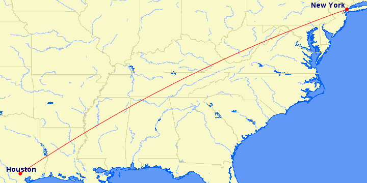
Houston to New York
The distance between the following two points \(([\phi_1,\lambda_1], [\phi_2,\lambda_2]) =([29.97, -95.35], [40.77, -73.98])\) (deg) is:
| Algorithm |
Procedure |
Result (meters) |
| Law of Cosines |
gcdist |
2272779.3057236285 |
| Haversine |
gcdist_haversine |
2272779.3057236294 |
| Vincenty |
gcdist_vincenty |
2272779.3057236290 |
Antipodal points
The distance between the following two antipodal points \(([\phi_1,\lambda_1], [\phi_2,\lambda_2]) = ([0, 0], [0.0, \pi/2])\) (radians) is:
| Algorithm |
Procedure |
Result (meters) |
| Law of Cosines |
gcdist |
20037508.342789244 |
| Haversine |
gcdist_haversine |
20037508.342789244 |
| Vincenty |
gcdist_vincenty |
20037508.342789244 |
Nearly antipodal points
The distance between the following two nearly antipodal points \(([\phi_1,\lambda_1], [\phi_2,\lambda_2]) = ([10^{-8}, 10^{-8}], [0.0, \pi/2])\) (radians) is:
| Algorithm |
Procedure |
Result (meters) |
| Law of Cosines |
gcdist |
20037508.342789244 |
| Haversine |
gcdist_haversine |
20037508.342789244 |
| Vincenty |
gcdist_vincenty |
20037508.252588764 |
Other methods
For a more accurate result, using an oblate-spheroid model of the Earth, the Vincenty inverse geodetic algorithm can be used (the equation above is just a special case of the more general algorithm when the ellipsoidal major and minor axes are equal). For the Houston to New York case, the difference between the spherical and oblate-spheroid equations is 282 meters.
See also
Feb 10, 2018
Many of the important algorithms we use today in the space business have their origins in NASA's Apollo program. For example, the Runge-Kutta methods with stepsize control developed by Erwin Fehlberg (1911-1990). These are still used today for propagating spacecraft trajectories. Fehlberg was a German mathematician who ended up at Marshall Spaceflight Center in Huntsville, Alabama. Many of the original reports documenting these methods are publicly available on the NASA Technical Reports Server (see references below). Modern Fortran implementations of Fehlberg's RK7(8) and RK8(9) methods (and others) can be found in the Fortran Astrodynamics Toolkit.
See also
- Fehlberg, E., "Classical Fifth-, Sixth-, Seventh-, and Eighth-Order Runge-Kutta Formulas with Stepsize Control", NASA-TR-R-287, 1968
- Fehlberg, E., "Low-order classical Runge-Kutta formulas with stepsize control and their application to some heat transfer problems", NASA-TR-R-315, 1969
- Fehlberg, E., "Classical eight- and lower-order Runge-Kutta-Nystrom formulas with stepsize control for special second-order differential equations", NASA-TR-R-381, M-533, 1972
- Fehlberg, E., "Classical eighth- and lower-order Runge-Kutta-Nystrom formulas with a new stepsize control procedure for special second-order differential equations", NASA-TR-R-410, M-544, 1973
- Fehlberg, E., "Classical seventh-, sixth-, and fifth-order Runge-Kutta-Nystrom formulas with stepsize control for general second-order differential equations", NASA-TR-R-432, M-546, 1974
Jan 27, 2018
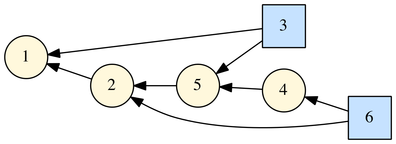
I released a new open source project on GitHub: DAGLIB, a modern Fortran library for manipulation of directed acyclic graphs (DAGs). This is based on some code I showed in a previous post. Right now, it's very basic, but you can use it to define DAGs, generate the topologically sorted order, and generate a "dot" file that can be used by GraphViz to visualize the DAG (such as the one shown at right).
In my recent AIAA paper I showed the following DAG representing how we have designed the upcoming Orion EM-1 mission:
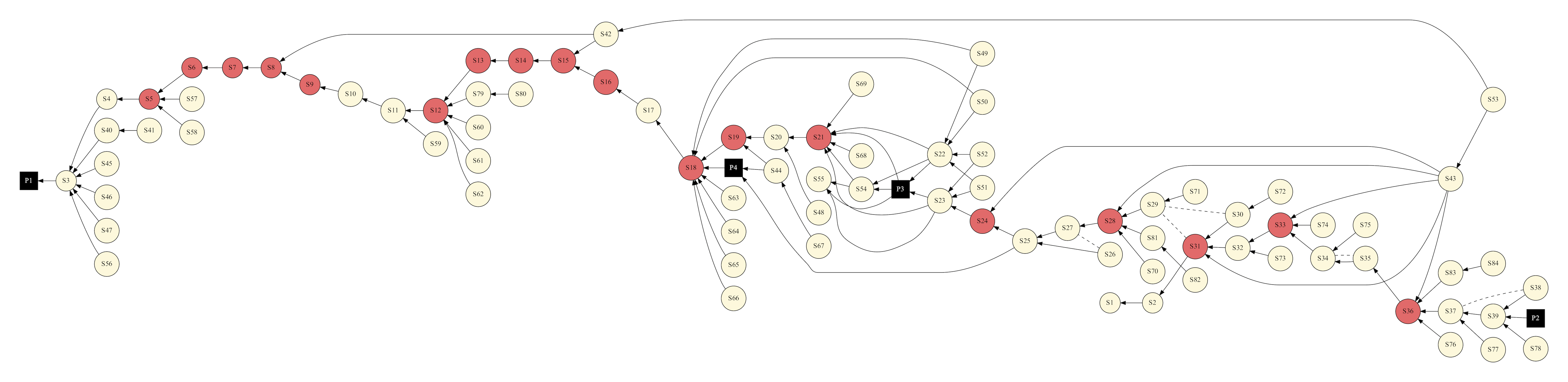

*During Exploration Mission-1, Orion will venture thousands of miles beyond the moon during an approximately three week mission. [NASA]*
In this case, the DAG represents the dependencies among different mission attributes (which represent maneuvers, coast phases, constraints, other algorithms, etc). To simulate the entire end-to-end mission, each element must be evaluated in the correct order such that all the dependencies are met. In this same paper, we also discuss other algorithms and their implementation in modern Fortran which may be familiar to readers of this blog.
See also
- J. Williams, R. D. Falck, and I. B. Beekman. "Application of Modern Fortran to Spacecraft Trajectory Design and Optimization", 2018 Space Flight Mechanics Meeting, AIAA SciTech Forum, (AIAA 2018-1451)
- (Modern?) Fortran directed graphs library [comp.lang.fortran] May 6, 2016
- JSON-Fortran GraphViz Example (how to generate a directed graph from a JSON structure), Apr 22, 2017
- The Ins and Outs of NASA’s First Launch of SLS and Orion, NASA, Nov. 27, 2015
Dec 12, 2016
In an earlier post, I mentioned that we needed an object-oriented modern Fortran library for multidimensional linear interpolation. Well, here it is. I call it finterp, and it is available on GitHub. It can be used for 1D-6D interpolation/extrapolation of data on a regular grid (i.e., not scattered). It has a similar object-oriented interface as my bspline-fortran library, with initialize, evaluate, and destroy methods like so:
type(linear_interp_3d) :: interp
call interp%initialize(xvec,yvec,zvec,fmat,iflag)
call interp%evaluate(x,y,z,f)
call interp%destroy()
For example, the low-level 3D interpolation evaluate routine is:
pure subroutine interp_3d(me,x,y,z,fxyz)

implicit none

class(linear_interp_3d),intent(inout) :: me
real(wp),intent(in) :: x
real(wp),intent(in) :: y
real(wp),intent(in) :: z
real(wp),intent(out) :: fxyz !! Interpolated ( f(x,y,z) )

integer,dimension(2) :: ix, iy, iz
real(wp) :: p1, p2, p3
real(wp) :: q1, q2, q3
integer :: mflag
real(wp) :: fx11, fx21, fx12, fx22, fxy1, fxy2

call dintrv(me%x,x,me%ilox,ix(1),ix(2),mflag)
call dintrv(me%y,y,me%iloy,iy(1),iy(2),mflag)
call dintrv(me%z,z,me%iloz,iz(1),iz(2),mflag)

q1 = (x-me%x(ix(1)))/(me%x(ix(2))-me%x(ix(1)))
q2 = (y-me%y(iy(1)))/(me%y(iy(2))-me%y(iy(1)))
q3 = (z-me%z(iz(1)))/(me%z(iz(2))-me%z(iz(1)))
p1 = one-q1
p2 = one-q2
p3 = one-q3

fx11 = p1*me%f(ix(1),iy(1),iz(1)) + q1*me%f(ix(2),iy(1),iz(1))
fx21 = p1*me%f(ix(1),iy(2),iz(1)) + q1*me%f(ix(2),iy(2),iz(1))
fx12 = p1*me%f(ix(1),iy(1),iz(2)) + q1*me%f(ix(2),iy(1),iz(2))
fx22 = p1*me%f(ix(1),iy(2),iz(2)) + q1*me%f(ix(2),iy(2),iz(2))
fxy1 = p2*( fx11 ) + q2*( fx21 )
fxy2 = p2*( fx12 ) + q2*( fx22 )

fxyz = p3*( fxy1 ) + q3*( fxy2 )

end subroutine interp_3d
The finterp library is released under a permissive BSD-3 license. As far as I can tell, it is unique among publicly-available Fortran codes in providing linear interpolation for up to 6D data sets. There used to be a Fortran 77 library called REGRIDPACK for regridding 1D-4D data sets (it had the option to use linear or cubic interpolation independently for each dimension). Written by John C. Adams at the National Center for Atmospheric Research in 1999, it used to be hosted at the UCAR website, but the link is now dead. You can still find it on the internet though, as part of other projects (for example here, where it is being used via a Python wrapper). But the licensing is unclear to me.
The dearth of easy-to-find, easy-to-use, high-quality open source modern Fortran libraries is a big problem for the long-term future of the language. Fortran users don't seem to be as interested in promoting their language as users of some of the newer programming languages are. There is a group of us working to change this, but we've got a long way to go. For example, Julia, a programming language only four years old, already has a ton of libraries, some of which are just wrappers to Fortran 77 code that no one's ever bothered to modernize. They even have a yearly conference. An in depth article about this state of affairs is a post for another day.
References
Dec 04, 2016

I present the initial release of a new modern Fortran library for computing Jacobian matrices using numerical differentiation. It is called NumDiff and is available on GitHub. The Jacobian is the matrix of partial derivatives of a set of \(m\) functions with respect to \(n\) variables:
$$
\mathbf{J}(\mathbf{x}) = \frac{d \mathbf{f}}{d \mathbf{x}} = \left[
\begin{array}{ c c c }
\frac{\partial f_1}{\partial x_1} & \cdots & \frac{\partial f_1}{\partial x_n} \\
\vdots & \ddots & \vdots \\
\frac{\partial f_m}{\partial x_1} & \cdots & \frac{\partial f_m}{\partial x_n} \\
\end{array}
\right]
$$
Typically, each variable \(x_i\) is perturbed by a value \(h_i\) using forward, backward, or central differences to compute the Jacobian one column at a time (\(\partial \mathbf{f} / \partial x_i\)). Higher-order methods are also possible [1]. The following finite difference formulas are currently available in the library:
- Two points:
- \((f(x+h)-f(x)) / h\)
- \((f(x)-f(x-h)) / h\)
- Three points:
- \((f(x+h)-f(x-h)) / (2h)\)
- \((-3f(x)+4f(x+h)-f(x+2h)) / (2h)\)
- \((f(x-2h)-4f(x-h)+3f(x)) / (2h)\)
- Four points:
- \((-2f(x-h)-3f(x)+6f(x+h)-f(x+2h)) / (6h)\)
- \((f(x-2h)-6f(x-h)+3f(x)+2f(x+h)) / (6h)\)
- \((-11f(x)+18f(x+h)-9f(x+2h)+2f(x+3h)) / (6h)\)
- \((-2f(x-3h)+9f(x-2h)-18f(x-h)+11f(x)) / (6h)\)
- Five points:
- \((f(x-2h)-8f(x-h)+8f(x+h)-f(x+2h)) / (12h)\)
- \((-3f(x-h)-10f(x)+18f(x+h)-6f(x+2h)+f(x+3h)) / (12h)\)
- \((-f(x-3h)+6f(x-2h)-18f(x-h)+10f(x)+3f(x+h)) / (12h)\)
- \((-25f(x)+48f(x+h)-36f(x+2h)+16f(x+3h)-3f(x+4h)) / (12h)\)
- \((3f(x-4h)-16f(x-3h)+36f(x-2h)-48f(x-h)+25f(x)) / (12h)\)
The basic features of NumDiff are listed here:
- A variety of finite difference methods are available (and it is easy to add new ones).
- If you want, you can specify a different finite difference method to use to compute each column of the Jacobian.
- You can also specify the number of points of the methods, and a suitable one of that order will be selected on-the-fly so as not to violate the variable bounds.
- I also included an alternate method using Neville's process which computes each element of the Jacobian individually [2]. It takes a very large number of function evaluations but produces the most accurate answer.
- A hash table based caching system is implemented to cache function evaluations to avoid unnecessary function calls if they are not necessary.
- It supports very large sparse systems by compactly storing and computing the Jacobian matrix using the sparsity pattern. Optimization codes such as SNOPT and Ipopt can use this form.
- It can also return the dense (\(m \times n\)) matrix representation of the Jacobian if that sort of thing is your bag (for example, the older SLSQP requires this form).
- It can also return the \(J*v\) product, where \(J\) is the full (\(m \times n\)) Jacobian matrix and v is an (\(n \times 1\)) input vector. This is used for Krylov type algorithms.
- The sparsity pattern can be supplied by the user or computed by the library.
- The sparsity pattern can also be partitioned so as compute multiple columns of the Jacobian simultaneously so as to reduce the number of function calls [3].
- It is written in object-oriented Fortran 2008. All user interaction is through a NumDiff class.
- It is open source with a BSD-3 license.
I haven't yet really tried to fine-tune the code, so I make no claim that it is the most optimal it could be. I'm using various modern Fortran vector and matrix intrinsic routines such as PACK, COUNT, etc. Likely there is room for efficiency improvements. I'd also like to add some parallelization, either using OpenMP or Coarray Fortran. OpenMP seems to have some issues with some modern Fortran constructs so that might be tricky. I keep meaning to do something real with coarrays, so this could be my chance.
So, there you go internet. If anybody else finds it useful, let me know.
References
- G. Engeln-Müllges, F. Uhlig, Numerical Algorithms with Fortran, Springer-Verlag Berlin Heidelberg, 1996.
- J. Oliver, "An algorithm for numerical differentiation of a function of one real variable", Journal of Computational and Applied Mathematics 6 (2) (1980) 145–160. [A Fortran 77 implementation of this algorithm by David Kahaner was formerly available from NIST, but the link seems to be dead. My modern Fortran version is available here.]
- T. F. Coleman, B. S. Garbow, J. J. Moré, "Algorithm 618: FORTRAN subroutines for estimating sparse Jacobian Matrices", ACM Transactions on Mathematical Software (TOMS), Volume 10 Issue 3, Sept. 1984.
Sep 24, 2016

The digits of \(\pi\) can be computed using the "Spigot algorithm" [1-2]. The interesting thing about this algorithm is that it doesn't use any floating point computations, only integers.
A Fortran version of the algorithm is given below (a translation of the Pascal program in the reference). It computes the first 10,000 digits of \(\pi\). The nines and predigit business is because the algorithm will occasionally output 10 as the next digit, and the 1 will need to be added to the previous digit. If we know in advance that this won't occur for a given range of digits, then the code can be greatly simplified. It can also be reformulated to compute multiple digits at a time if we change the base (see [1] for the simplified version in base 10,000).
subroutine compute_pi()

    implicit none

    integer, parameter :: n = 10000 ! number of digits to compute
    integer, parameter :: len = 10*n/3 + 1

    integer :: i, j, k, q, x, nines, predigit
    integer, dimension(len) :: a

    a = 2
    nines = 0
    predigit = 0

    do j = 1, n
        q = 0
        do i = len, 1, -1
            x = 10*a(i) + q*i
            a(i) = mod(x, 2*i - 1)
            q = x/(2*i - 1)
        end do
        a(1) = mod(q, 10)
        q = q/10
        if (q == 9) then
            nines = nines + 1
        else if (q == 10) then
            write (*, '(I1)', advance='NO') predigit + 1
            do k = 1, nines
                write (*, '(I1)', advance='NO') 0
            end do
            predigit = 0
            nines = 0
        else
            if (j == 2) then
                write (*, '(I1,".")', advance='NO') predigit
            else if (j /= 1) then
                write (*, '(I1)', advance='NO') predigit
            end if
            predigit = q
            if (nines /= 0) then
            do k = 1, nines
                write (*, '(I1)', advance='NO') 9
            end do
            nines = 0
            end if
        end if
    end do
    write (*, '(I1)', advance='NO') predigit

end subroutine compute_pi
The algorithm as originally published contained a mistake (len = 10*n/3). The correction is due to [3]. The code above produces the following output:
3.141592653589793238462643383279502884197169399375105820974944592307816406286208998628034825342117067982148086513282306647093844609550582231725359408128481117450284102701938521105559644622948954930381964428810975665933446128475648233786783165271201909145648566923460348610454326648213393607260249141273724587006606315588174881520920962829254091715364367892590360011330530548820466521384146951941511609433057270365759591953092186117381932611793105118548074462379962749567351885752724891227938183011949129833673362440656643086021394946395224737190702179860943702770539217176293176752384674818467669405132000568127145263560827785771342757789609173637178721468440901224953430146549585371050792279689258923542019956112129021960864034418159813629774771309960518707211349999998372978049951059731732816096318595024459455346908302642522308253344685035261931188171010003137838752886587533208381420617177669147303598253490428755468731159562863882353787593751957781857780532171226806613001927876611195909216420198938095257201065485863278865936153381827968230301952035301852968995773622599413891249721775283479131515574857242454150695950829533116861727855889075098381754637464939319255060400927701671139009848824012858361603563707660104710181942955596198946767837449448255379774726847104047534646208046684259069491293313677028989152104752162056966024058038150193511253382430035587640247496473263914199272604269922796782354781636009341721641219924586315030286182974555706749838505494588586926995690927210797509302955321165344987202755960236480665499119881834797753566369807426542527862551818417574672890977772793800081647060016145249192173217214772350141441973568548161361157352552133475741849468438523323907394143334547762416862518983569485562099219222184272550254256887671790494601653466804988627232791786085784383827967976681454100953883786360950680064225125205117392984896084128488626945604241965285022210661186306744278622039194945047123713786960956364371917287467764657573962413890865832645995813390478027590099465764078951269468398352595709825822620522489407726719478268482601476990902640136394437455305068203496252451749399651431429809190659250937221696461515709858387410597885959772975498930161753928468138268683868942774155991855925245953959431049972524680845987273644695848653836736222626099124608051243884390451244136549762780797715691435997700129616089441694868555848406353422072225828488648158456028506016842739452267467678895252138522549954666727823986456596116354886230577456498035593634568174324112515076069479451096596094025228879710893145669136867228748940560101503308617928680920874760917824938589009714909675985261365549781893129784821682998948722658804857564014270477555132379641451523746234364542858444795265867821051141354735739523113427166102135969536231442952484937187110145765403590279934403742007310578539062198387447808478489683321445713868751943506430218453191048481005370614680674919278191197939952061419663428754440643745123718192179998391015919561814675142691239748940907186494231961567945208095146550225231603881930142093762137855956638937787083039069792077346722182562599661501421503068038447734549202605414665925201497442850732518666002132434088190710486331734649651453905796268561005508106658796998163574736384052571459102897064140110971206280439039759515677157700420337869936007230558763176359421873125147120532928191826186125867321579198414848829164470609575270695722091756711672291098169091528017350671274858322287183520935396572512108357915136988209144421006751033467110314126711136990865851639831501970165151168517143765761835155650884909989859982387345528331635507647918535893226185489632132933089857064204675259070915481416549859461637180270981994309924488957571282890592323326097299712084433573265489382391193259746366730583604142813883032038249037589852437441702913276561809377344403070746921120191302033038019762110110044929321516084244485963766983895228684783123552658213144957685726243344189303968642624341077322697802807318915441101044682325271620105265227211166039666557309254711055785376346682065310989652691862056476931257058635662018558100729360659876486117910453348850346113657686753249441668039626579787718556084552965412665408530614344431858676975145661406800700237877659134401712749470420562230538994561314071127000407854733269939081454664645880797270826683063432858785698305235808933065757406795457163775254202114955761581400250126228594130216471550979259230990796547376125517656751357517829666454779174501129961489030463994713296210734043751895735961458901938971311179042978285647503203198691514028708085990480109412147221317947647772622414254854540332157185306142288137585043063321751829798662237172159160771669254748738986654949450114654062843366393790039769265672146385306736096571209180763832716641627488880078692560290228472104031721186082041900042296617119637792133757511495950156604963186294726547364252308177036751590673502350728354056704038674351362222477158915049530984448933309634087807693259939780541934144737744184263129860809988868741326047215695162396586457302163159819319516735381297416772947867242292465436680098067692823828068996400482435403701416314965897940924323789690706977942236250822168895738379862300159377647165122893578601588161755782973523344604281512627203734314653197777416031990665541876397929334419521541341899485444734567383162499341913181480927777103863877343177207545654532207770921201905166096280490926360197598828161332316663652861932668633606273567630354477628035045077723554710585954870279081435624014517180624643626794561275318134078330336254232783944975382437205835311477119926063813346776879695970309833913077109870408591337464144282277263465947047458784778720192771528073176790770715721344473060570073349243693113835049316312840425121925651798069411352801314701304781643788518529092854520116583934196562134914341595625865865570552690496520985803385072242648293972858478316305777756068887644624824685792603953527734803048029005876075825104747091643961362676044925627420420832085661190625454337213153595845068772460290161876679524061634252257719542916299193064553779914037340432875262888963995879475729174642635745525407909145135711136941091193932519107602082520261879853188770584297259167781314969900901921169717372784768472686084900337702424291651300500516832336435038951702989392233451722013812806965011784408745196012122859937162313017114448464090389064495444006198690754851602632750529834918740786680881833851022833450850486082503930213321971551843063545500766828294930413776552793975175461395398468339363830474611996653858153842056853386218672523340283087112328278921250771262946322956398989893582116745627010218356462201349671518819097303811980049734072396103685406643193950979019069963955245300545058068550195673022921913933918568034490398205955100226353536192041994745538593810234395544959778377902374216172711172364343543947822181852862408514006660443325888569867054315470696574745855033232334210730154594051655379068662733379958511562578432298827372319898757141595781119635833005940873068121602876496286744604774649159950549737425626901049037781986835938146574126804925648798556145372347867330390468838343634655379498641927056387293174872332083760112302991136793862708943879936201629515413371424892830722012690147546684765357616477379467520049075715552781965362132392640616013635815590742202020318727760527721900556148425551879253034351398442532234157623361064250639049750086562710953591946589751413103482276930624743536325691607815478181152843667957061108615331504452127473924544945423682886061340841486377670096120715124914043027253860764823634143346235189757664521641376796903149501910857598442391986291642193994907236234646844117394032659184044378051333894525742399508296591228508555821572503107125701266830240292952522011872676756220415420516184163484756516999811614101002996078386909291603028840026910414079288621507842451670908700069928212066041837180653556725253256753286129104248776182582976515795984703562226293486003415872298053498965022629174878820273420922224533985626476691490556284250391275771028402799806636582548892648802545661017296702664076559042909945681506526530537182941270336931378517860904070866711496558343434769338578171138645587367812301458768712660348913909562009939361031029161615288138437909904231747336394804575931493140529763475748119356709110137751721008031559024853090669203767192203322909433467685142214477379393751703443661991040337511173547191855046449026365512816228824462575916333039107225383742182140883508657391771509682887478265699599574490661758344137522397096834080053559849175417381883999446974867626551658276584835884531427756879002909517028352971634456212964043523117600665101241200659755851276178583829204197484423608007193045761893234922927965019875187212726750798125547095890455635792122103334669749923563025494780249011419521238281530911407907386025152274299581807247162591668545133312394804947079119153267343028244186041426363954800044800267049624820179289647669758318327131425170296923488962766844032326092752496035799646925650493681836090032380929345958897069536534940603402166544375589004563288225054525564056448246515187547119621844396582533754388569094113031509526179378002974120766514793942590298969594699556576121865619673378623625612521632086286922210327488921865436480229678070576561514463204692790682120738837781423356282360896320806822246801224826117718589638140918390367367222088832151375560037279839400415297002878307667094447456013455641725437090697939612257142989467154357846878861444581231459357198492252847160504922124247014121478057345510500801908699603302763478708108175450119307141223390866393833952942578690507643100638351983438934159613185434754649556978103829309716465143840700707360411237359984345225161050702705623526601276484830840761183013052793205427462865403603674532865105706587488225698157936789766974220575059683440869735020141020672358502007245225632651341055924019027421624843914035998953539459094407046912091409387001264560016237428802109276457931065792295524988727584610126483699989225695968815920560010165525637567
See also
- S. Rabinowitz, Abstract 863–11–482: A Spigot Algorithm for Pi, American Mathematical Society, 12(1991)30, 1991.
- S. Rabinowitz, S. Wagon, "A Spigot Algorithm for the Digits of \(\pi\)", American Mathematical Monthly, Vol. 102, Issue 3, March 1995, p. 195-203.
- J. Arndt, C. Haenel, π Unleashed, Springer, 2000.
Jan 31, 2016

*Thaddeus Vincenty (1920--2002) Image source: [IAG Newsletter](http://www.gfy.ku.dk/~iag/newslett/news7606.htm)*
There are two standard problems in geodesy:
- Direct geodetic problem -- Given a point on the Earth (latitude and longitude) and the direction (azimuth) and distance from that point to a second point, determine the latitude and longitude of that second point.
- Inverse geodetic problem -- Given two points on the Earth, determine the azimuth and distance between them.
Assuming the Earth is an oblate spheroid, both of these can be solved using the iterative algorithms by Thaddeus Vincenty [1]. Modern Fortran versions of Vincenty's algorithms can be found in the geodesy module of the Fortran Astrodynamics Toolkit [2].
The direct algorithm was listed in an earlier post. If we assume a WGS84 Earth ellipsoid (a=6378.137 km, f=1/298.257223563), an example direct calculation is:
$$
\begin{array}{rcll}
\phi_1 &= & 29.97^{\circ} & \mathrm{(Latitude ~of ~ first ~ point)}\\
\lambda_1 &= & -95.35^{\circ} & \mathrm{(Longitude ~of ~ first ~point)} \\
Az &= & 20^{\circ} & \mathrm{(Azimuth)}\\
s &= & 50~\mathrm{km} & \mathrm{(Distance)}
\end{array}
$$
The latitude and longitude of the second point is:
$$
\begin{array}{rcl}
\phi_2 &= & 30.393716^{\circ} \\
\lambda_2 &= & -95.172057^{\circ} \\
\end{array}
$$
The more complicated inverse algorithm is listed here (based on the USNGS code from [1]):
subroutine inverse(a, rf, b1, l1, b2, l2, faz, baz, s, it, sig, lam, kind)

    use, intrinsic :: iso_fortran_env, wp => real64

    implicit none

    real(wp), intent(in) :: a !! Equatorial semimajor axis
    real(wp), intent(in) :: rf !! reciprocal flattening (1/f)
    real(wp), intent(in) :: b1 !! latitude of point 1 (rad, positive north)
    real(wp), intent(in) :: l1 !! longitude of point 1 (rad, positive east)
    real(wp), intent(in) :: b2 !! latitude of point 2 (rad, positive north)
    real(wp), intent(in) :: l2 !! longitude of point 2 (rad, positive east)
    real(wp), intent(out) :: faz !! Forward azimuth (rad, clockwise from north)
    real(wp), intent(out) :: baz !! Back azimuth (rad, clockwise from north)
    real(wp), intent(out) :: s !! Ellipsoidal distance
    integer, intent(out) :: it !! iteration count
    real(wp), intent(out) :: sig !! spherical distance on auxiliary sphere
    real(wp), intent(out) :: lam !! longitude difference on auxiliary sphere
    integer, intent(out) :: kind !! solution flag: kind=1, long-line; kind=2, antipodal

    real(wp) :: beta1, beta2, biga, bigb, bige, bigf, boa, &
                c, cosal2, coslam, cossig, costm, costm2, &
                cosu1, cosu2, d, dsig, ep2, l, prev, sinal, &
                sinlam, sinsig, sinu1, sinu2, tem1, tem2, &
                temp, test, z

    real(wp), parameter :: pi = acos(-1.0_wp)
    real(wp), parameter :: two_pi = 2.0_wp*pi
    real(wp), parameter :: tol = 1.0e-14_wp !! convergence tolerance
    real(wp), parameter :: eps = 1.0e-15_wp !! tolerance for zero

    boa = 1.0_wp - 1.0_wp/rf

    beta1 = atan(boa*tan(b1))
    sinu1 = sin(beta1)
    cosu1 = cos(beta1)
    beta2 = atan(boa*tan(b2))
    sinu2 = sin(beta2)
    cosu2 = cos(beta2)

    l = l2 - l1
    if (l > pi) l = l - two_pi
    if (l < -pi) l = l + two_pi
    prev = l
    test = l
    it = 0
    kind = 1
    lam = l

    longline: do ! long-line loop (kind=1)

        sinlam = sin(lam)
        coslam = cos(lam)
        temp = cosu1*sinu2 - sinu1*cosu2*coslam
        sinsig = sqrt((cosu2*sinlam)**2 + temp**2)
        cossig = sinu1*sinu2 + cosu1*cosu2*coslam
        sig = atan2(sinsig, cossig)
        if (abs(sinsig) < eps) then
            sinal = cosu1*cosu2*sinlam/sign(eps, sinsig)
        else
            sinal = cosu1*cosu2*sinlam/sinsig
        end if
        cosal2 = -sinal**2 + 1.0_wp
        if (abs(cosal2) < eps) then
            costm = -2.0_wp*(sinu1*sinu2/sign(eps, &
                                              cosal2)) + cossig
        else
            costm = -2.0_wp*(sinu1*sinu2/cosal2) + &
                    cossig
        end if
        costm2 = costm*costm
        c = ((-3.0_wp*cosal2 + 4.0_wp)/rf + 4.0_wp)* &
            cosal2/rf/16.0_wp

        antipodal: do ! antipodal loop (kind=2)

            it = it + 1
            d = (((2.0_wp*costm2 - 1.0_wp)*cossig*c + &
                  costm)*sinsig*c + sig)*(1.0_wp - c)/rf
            if (kind == 1) then
                lam = l + d*sinal
                if (abs(lam - test) >= tol) then
                    if (abs(lam) > pi) then
                        kind = 2
                        lam = pi
                        if (l < 0.0_wp) lam = -lam
                        sinal = 0.0_wp
                        cosal2 = 1.0_wp
                        test = 2.0_wp
                        prev = test
                        sig = pi - abs(atan(sinu1/cosu1) + &
                                    atan(sinu2/cosu2))
                        sinsig = sin(sig)
                        cossig = cos(sig)
                        c = ((-3.0_wp*cosal2 + 4.0_wp)/rf + &
                            4.0_wp)*cosal2/rf/16.0_wp
                        if (abs(sinal - prev) < tol) exit longline
                        if (abs(cosal2) < eps) then
                            costm = -2.0_wp*(sinu1*sinu2/ &
                                            sign(eps, cosal2)) + cossig
                        else
                            costm = -2.0_wp*(sinu1*sinu2/cosal2) + &
                                    cossig
                        end if
                        costm2 = costm*costm
                        cycle antipodal
                    end if
                    if (((lam - test)*(test - prev)) < 0.0_wp .and. it > 5) &
                        lam = (2.0_wp*lam + 3.0_wp*test + prev)/6.0_wp
                    prev = test
                    test = lam
                    cycle longline
                end if
            else
                sinal = (lam - l)/d
                if (((sinal - test)*(test - prev)) < 0.0_wp .and. it > 5) &
                    sinal = (2.0_wp*sinal + 3.0_wp*test + prev)/6.0_wp
                prev = test
                test = sinal
                cosal2 = -sinal**2 + 1.0_wp
                sinlam = sinal*sinsig/(cosu1*cosu2)
                coslam = -sqrt(abs(-sinlam**2 + 1.0_wp))
                lam = atan2(sinlam, coslam)
                temp = cosu1*sinu2 - sinu1*cosu2*coslam
                sinsig = sqrt((cosu2*sinlam)**2 + temp**2)
                cossig = sinu1*sinu2 + cosu1*cosu2*coslam
                sig = atan2(sinsig, cossig)
                c = ((-3.0_wp*cosal2 + 4.0_wp)/rf + 4.0_wp)* &
                    cosal2/rf/16.0_wp
                if (abs(sinal - prev) >= tol) then
                if (abs(cosal2) < eps) then
                    costm = -2.0_wp*(sinu1*sinu2/ &
                                     sign(eps, cosal2)) + cossig
                else
                    costm = -2.0_wp*(sinu1*sinu2/cosal2) + &
                            cossig
                end if
                costm2 = costm*costm
                cycle antipodal
                end if
            end if

            exit longline

        end do antipodal

    end do longline

    if (kind == 2) then ! antipodal
        faz = sinal/cosu1
        baz = sqrt(-faz**2 + 1.0_wp)
        if (temp < 0.0_wp) baz = -baz
        faz = atan2(faz, baz)
        tem1 = -sinal
        tem2 = sinu1*sinsig - cosu1*cossig*baz
        baz = atan2(tem1, tem2)
    else ! long-line
        tem1 = cosu2*sinlam
        tem2 = cosu1*sinu2 - sinu1*cosu2*coslam
        faz = atan2(tem1, tem2)
        tem1 = -cosu1*sinlam
        tem2 = sinu1*cosu2 - cosu1*sinu2*coslam
        baz = atan2(tem1, tem2)
    end if

    if (faz < 0.0_wp) faz = faz + two_pi
    if (baz < 0.0_wp) baz = baz + two_pi
    ep2 = 1.0_wp/(boa*boa) - 1.0_wp
    bige = sqrt(1.0_wp + ep2*cosal2)
    bigf = (bige - 1.0_wp)/(bige + 1.0_wp)
    biga = (1.0_wp + bigf*bigf/4.0_wp)/(1.0_wp - bigf)
    bigb = bigf*(1.0_wp - 0.375_wp*bigf*bigf)
    z = bigb/6.0_wp*costm*(-3.0_wp + 4.0_wp* &
                           sinsig**2)*(-3.0_wp + 4.0_wp*costm2)
    dsig = bigb*sinsig*(costm + bigb/4.0_wp* &
                        (cossig*(-1.0_wp + 2.0_wp*costm2) - z))
    s = (boa*a)*biga*(sig - dsig)

end subroutine inverse
For the same ellipsoid, an example inverse calculation is:
$$
\begin{array}{rcll}
\phi_1 &= & 29.97^{\circ} & \mathrm{(Latitude ~of ~ first ~ point)}\\
\lambda_1 &= & -95.35^{\circ} & \mathrm{(Longitude ~of ~ first ~point)} \\
\phi_2 &= & 40.77^{\circ} & \mathrm{(Latitude ~of ~ second ~ point)}\\
\lambda_2 &= & -73.98^{\circ} & \mathrm{(Longitude ~of ~ second ~point)}
\end{array}
$$
The azimuth and distance from the first to the second point is:
$$
\begin{array}{rcl}
Az &= & 52.400056^{\circ} & \mathrm{(Azimuth)}\\
s &= & 2272.497~\mathrm{km} & \mathrm{(Distance)}
\end{array}
$$
References