Degenerate Conic

SLSQP

Rosenbrock function generated by Grapher.

SLSQP [1-2] is a sequential quadratic programming (SQP) optimization algorithm written by Dieter Kraft in the 1980s. It can be used to solve nonlinear programming problems that minimize a scalar function:

$$ f(\mathbf{x}) $$

subject to general equality and inequality constraints:

$$ \begin{array}{rl} g_j(\mathbf{x}) = \mathbf{0} & j = 1, \dots ,m_e \\ g_j(\mathbf{x}) \ge \mathbf{0} & j = m_e+1, \dots ,m \end{array} $$

and to lower and upper bounds on the variables:

$$ \begin{array}{rl} l_i \le x_i \le u_i & i = 1, \dots ,n \end{array} $$

SLSQP was written in Fortran 77, and is included in PyOpt (called using Python wrappers) and NLopt (as an f2c translation of the original source). It is also included as one of the solvers in two of NASA's trajectory optimization tools (OTIS and Copernicus).

The code is pretty old school and includes numerous obsolescent Fortran features such as arithmetic IF statements, computed and assigned GOTO statements, statement functions, etc. It also includes some non-standard assumptions (implicit saving of variables and initialization to zero).

So, the time is ripe for refactoring SLSQP. Which is what I've done. The refactored version includes some new features and bug fixes, including:

It is now thread safe. The original version was not thread safe due to the use of saved variables in one of the subroutines.
It should now be 100% standard compliant (Fortran 2008).
It now has an easy-to-use object-oriented interface. The slsqp_class is used for all interactions with the solver. Methods include initialize(), optimize(), and destroy().
It includes updated versions of some of the third-party routines used in the original code (BLAS, LINPACK, and NNLS).
It has been translated into free-form source. For this, I used the sample online version of the SPAG Fortran Code Restructuring tool to perform some of the translation, which seemed to work really well. The rest I did manually. Fixed-form source (FORTRAN 77 style) is terrible and needs to die. There's no reason to be using it 25 years after the introduction of free-form source (yes, I'm talking to you Claus 😀).
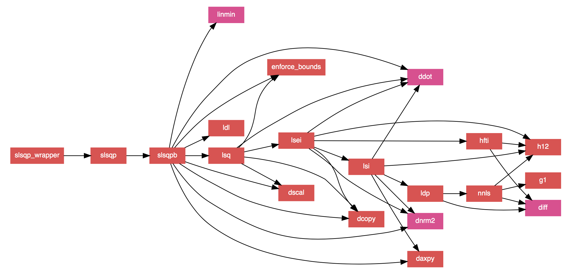
The documentation strings in the code have been converted to FORD format, allowing for nicely formatted documentation to be auto-generated (which includes MathJax formatted equations to replace the ASCII ones in the original code). It also generates ultra-slick call graphs like the one below.
A couple of bug fixes noted elsewhere have been applied (see here and here).

SLSQP call graph generated by FORD.

The original code used a "reverse communication" interface, which was one of the workarounds used in old Fortran code to make up for the fact that there wasn't really a good way to pass arbitrary data into a library routine. So, the routine returns after called, requests data, and then is called again. For now, I've kept the reverse communication interface in the core routines (the user never interacts with them directly, however). Eventually, I may do away with this, since I don't think it's particularly useful anymore.

The new code is on GitHub, and is released under a BSD license. There are various additional improvements that could be made, so I'll continue to tinker with it, but for now it seems to work fine. If anyone else finds the new version useful, I'd be interested to hear about it.

Conversion Factors

1 lbm = 0.45359237 kg
1 lbf = 4.4482216152605 N
1 ft = 0.3048 m
1 mile = 1.609344 km
1 nmi = 1.852 km
1 slug = 1 $\mathrm{lbf} ~ \mathrm{s}^2 / \mathrm{ft} \approx$ 14.5939029 kg

References

Fortran Code

module conversion_factors

use, intrinsic :: iso_fortran_env, only: wp => real64 !double precision

implicit none

real(wp),parameter :: one = 1.0_wp

real(wp),parameter :: lbm2kg = 0.45359237_wp     ! exact
real(wp),parameter :: lbf2N = 4.4482216152605_wp !
real(wp),parameter :: ft2m = 0.3048_wp           !
real(wp),parameter :: mile2km = 1.609344_wp      !
real(wp),parameter :: nmi2km = 1.852_wp          !
real(wp),parameter :: slug2kg = lbf2N/ft2m       ! ~ 14.593902937206362

real(wp),parameter :: kg2lbm = one/lbm2kg        ! ~ 2.2046226218487757
real(wp),parameter :: N2lbf = one/lbf2N          ! ~ 0.2248089430997105
real(wp),parameter :: m2ft = one/ft2m            ! ~ 3.280839895013123
real(wp),parameter :: km2mile = one/mile2km      ! ~ 0.621371192237334
real(wp),parameter :: km2nmi = one/nmi2km        ! ~ 0.5399568034557235
real(wp),parameter :: kg2slug = one/slug2kg      ! ~ 0.06852176585679176

end module conversion_factors

posted at 17:07 · Algorithms · Fortran NIST Units

Complex Step Differentiation

Complex step differentiation is a method for estimating the derivative of a function $f(x)$ using the equation:

$f'(x) \approx \frac{ Im[f(x + ih)] }{h}$

Unlike finite-difference formulas, the complex-step formula does not suffer from roundoff errors due to subtraction, so a very small value of the step size $h$ can be used, producing a much more accurate derivative. The example shown below is for the function: $f(x) = e^x + \sin(x)$. The derivative error is compared to three finite-difference formulas:

$f'(x) \approx \frac{f(x+h) - f(x)}{h}$ (Two-point forward difference)
$f'(x) \approx \frac{f(x+h) - f(x-h)}{2h}$ (Two-point central difference)
$f'(x) \approx \frac{f(x-2h) -8 f(x-h) + 8 f(x+h) - f(x+2h) }{12 h}$ (Four-point central difference)

For large values of $h$, truncation error dominates. The finite-difference error decreases as $h$ is decreased, until roundoff error begins to dominate (around $10^{-8}$ for the forward difference, $10^{-5}$ for the 2-point central difference, and $10^{-3}$ for the 4-point central difference). The complex-step estimate, however, can produce a derivative estimate to machine precision for any value of $h < 10^{-8}$.

Algorithms • Modern Fortran Programming • Orbital Mechanics

Jan 12, 2016

SLSQP

See Also

Mar 21, 2015

Conversion Factors

Conversion Factors

References

Fortran Code

Nov 03, 2014

Complex Step Differentiation

See also