Jun 14, 2026
The FMIN function at Netlib is based on Richard Brent's classic localmin algorithm from [1].
The method uses a combination of golden section search and successive parabolic interpolation to compute the minimum of a 1D function without the necessity of evaluating any derivatives. There are Fortran 66 and ALGOL 60 versions of the method in the reference. I also have a modernized version here.
Let's show an example of how to use it for a simple orbital mechanics application.
Problem setup
Let's solve a trivial problem in orbital mechanics: computing the time of closest approach to a planet for a conic orbit. This is known as periapsis (or, for the Earth, perigee). We don't really need to use a minimizer to compute this, but it's a problem with a known solution that we can test the minimizer on.
We need various algorithms to do this:
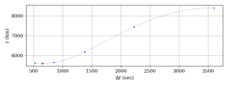
Given an initial elliptical orbit state, the Gooding routine pv3els will compute the time since last periapsis passage, so we have the "true" value to compare the results against. The function we pass to fmin to minimize will simply propagate the state (the independent variable is \(\Delta t\)) and return the radius magnitude (\(r\)). The point where the radius magnitude is minimized is the periapsis point we are looking for. The orbital period is used to set the upper time bound for the minimizer (we know there is only one periapsis passage per orbital period).
Example code
In our Fortran Package Manager manifest file, we define the two external dependencies we need:
[dependencies]
fmin = { git="https://github.com/jacobwilliams/fmin.git" }
fortran-astrodynamics-toolkit = { git="https://github.com/jacobwilliams/fortran-astrodynamics-toolkit.git" }
And the main program looks like this:
program main
  use fmin_module, wp => fmin_rk
  use fortran_astrodynamics_toolkit

  implicit none

  real(wp) :: p !! semiparameter [km]
  real(wp) :: period !! orbital period [sec]
  real(wp) :: dt !! time from initial state to periapsis [sec]
  real(wp),dimension(3) :: r, v !! position and velocity vectors [km] and [km/s]
  real(wp),dimension(6) :: rv0 !! initial state vector [km, km/s]
  real(wp),dimension(6) :: e0 !! Gooding orbital elements of the initial state
  integer :: n_evals = 0 !! number of function evaluations

  ! initial conditions (orbital elements):
  real(wp),parameter :: mu   = 398600.4418_wp  !! Earth grav. parameter [km^3/s^2]
  real(wp),parameter :: a    = 7000.0_wp       !! semi-major axis [km]
  real(wp),parameter :: ecc  = 0.2_wp          !! eccentricity
  real(wp),parameter :: inc  = 30.0_wp         !! inclination [deg]
  real(wp),parameter :: raan = 40.0_wp         !! right ascension of ascending node [deg]
  real(wp),parameter :: aop  = 60.0_wp         !! argument of perigee [deg]
  real(wp),parameter :: tru  = -45.0_wp        !! true anomaly [deg]
  real(wp),parameter :: tol  = 1.0e-6_wp       !! tolerance for fmin

  ! get the initial state vector and time from periapsis for the initial state:
  p = a * (1.0_wp - ecc**2)
  period = orbit_period(mu,a)
  call orbital_elements_to_rv(mu, p, ecc, inc, raan, aop, tru, r, v)
  rv0 = [r, v]
  call pv3els (mu, rv0, e0) ! e0(6) is the time from periapsis of the initial state

  ! call the minimizer:
  dt = fmin(func,0.0_wp,period,tol)

  ! print results
  write(*,'(A,F12.6,A)') 'DT to periapsis from fmin        = ', dt, ' sec'
  write(*,'(A,F12.6,A)') 'True initial time from periapsis = ', e0(6), ' sec'
  write(*,'(A,E12.3,A)') 'Error                            = ', dt + e0(6), ' sec'
  write(*,'(A,I0,A)')    'number of function evals         = ', n_evals, ' '

  contains

  function func(x) result(f)
    !! the function is to propagate from the initial state
    !! by the dt and compute the radius value
    real(wp),intent(in) :: x  !! indep. variable (dt)
    real(wp)            :: f  !! function value `f(x)` - radius magnitude
    real(wp),dimension(6) :: rvf
    call propagate(mu, rv0, x, rvf)
    f = norm2(rvf(1:3))
    n_evals = n_evals + 1
  end function func

end program main
Easy peasy!
Results
The result of running this program is:
DT to periapsis from fmin        =   652.983248 sec
True initial time from periapsis =  -652.983240 sec
Error                            =    0.875E-05 sec
number of function evals         = 12
So, it works! Using 12 function evaluations (i.e., kepler propagations of the orbit), the method has located the periapsis time to within about 8 \(\mu s\).
This sort of approach can also be used for less-trivial problems where we don't have a good analytical solution, and/or derivatives are unavailable or hard to obtain.
References
- R. Brent, "Algorithms for Minimization Without Derivatives", Prentice-Hall, 1973.
Sep 15, 2019
I'm working on a modern Fortran version of the simulated annealing optimization algorithm, using this code as a starting point. There is a Fortran 90 version here, but this seems to be mostly just a straightforward conversion of the original code to free-form source formatting. I have in mind a more thorough modernization and the addition of some new features that I need.
Refactoring old Fortran code is always fun. Consider the following snippet:
C  Check termination criteria.
      QUIT = .FALSE.
      FSTAR(1) = F
      IF ((FOPT - FSTAR(1)) .LE. EPS) QUIT = .TRUE.
      DO 410, I = 1, NEPS
        IF (ABS(F - FSTAR(I)) .GT. EPS) QUIT = .FALSE.
410   CONTINUE
This can be greatly simplified to:
! check termination criteria.
fstar(1) = f
quit = ((fopt-f)<=eps) .and. (all(abs(f-fstar)<=eps)
Note that we are using some of the vector features of modern Fortran to remove the loop. Consider also this function in the original code:
      FUNCTION  EXPREP(RDUM)
C  This function replaces exp to avoid under- and overflows and is
C  designed for IBM 370 type machines. It may be necessary to modify
C  it for other machines. Note that the maximum and minimum values of
C  EXPREP are such that they has no effect on the algorithm.

      DOUBLE PRECISION  RDUM, EXPREP

      IF (RDUM .GT. 174.) THEN
         EXPREP = 3.69D+75
      ELSE IF (RDUM .LT. -180.) THEN
         EXPREP = 0.0
      ELSE
         EXPREP = EXP(RDUM)
      END IF

      RETURN
      END
It is somewhat disturbing that the comments mention IBM 370 machines. This routine is unchanged in the f90 version. However, these numeric values are no longer correct for modern hardware. Using modern Fortran, we can write a totally portable version of this routine like so:
pure function exprep(x) result(f)

use, intrinsic :: ieee_exceptions

implicit none

real(dp), intent(in) :: x
real(dp) :: f

logical,dimension(2) :: flags
type(ieee_flag_type),parameter,dimension(2) :: out_of_range = [ieee_overflow,ieee_underflow]

call ieee_set_halting_mode(out_of_range,.false.)

f = exp(x)

call ieee_get_flag(out_of_range,flags)
if (any(flags)) then
  call ieee_set_flag(out_of_range,.false.)
  if (flags(1)) then
    f = huge(1.0_dp)
  else
    f = 0.0_dp
  end if
end if

end function exprep
This new version is entirely portable and works for any real kind. It contains no magic numbers and uses the intrinsic IEEE exceptions module of modern Fortran to protect against overflow and underflow, and the huge() intrinsic to return the largest real(dp) number.
So, stay tuned...
See also
- S. Kirkpatrick, C. D. Gelatt Jr., M. P. Vecchi, "Optimization by Simulated Annealing", Science 13 May 1983, Vol. 220, Issue 4598, pp. 671-680
- W. L. Goffe, SIMANN: A Global Optimization Algorithm using Simulated Annealing, Studies in Nonlinear Dynamics & Econometrics, De Gruyter, vol. 1(3), pages 1-9, October 1996.
- Original simann.f source code [Netlib]
Dec 04, 2016

I present the initial release of a new modern Fortran library for computing Jacobian matrices using numerical differentiation. It is called NumDiff and is available on GitHub. The Jacobian is the matrix of partial derivatives of a set of \(m\) functions with respect to \(n\) variables:
$$
\mathbf{J}(\mathbf{x}) = \frac{d \mathbf{f}}{d \mathbf{x}} = \left[
\begin{array}{ c c c }
\frac{\partial f_1}{\partial x_1} & \cdots & \frac{\partial f_1}{\partial x_n} \\
\vdots & \ddots & \vdots \\
\frac{\partial f_m}{\partial x_1} & \cdots & \frac{\partial f_m}{\partial x_n} \\
\end{array}
\right]
$$
Typically, each variable \(x_i\) is perturbed by a value \(h_i\) using forward, backward, or central differences to compute the Jacobian one column at a time (\(\partial \mathbf{f} / \partial x_i\)). Higher-order methods are also possible [1]. The following finite difference formulas are currently available in the library:
- Two points:
- \((f(x+h)-f(x)) / h\)
- \((f(x)-f(x-h)) / h\)
- Three points:
- \((f(x+h)-f(x-h)) / (2h)\)
- \((-3f(x)+4f(x+h)-f(x+2h)) / (2h)\)
- \((f(x-2h)-4f(x-h)+3f(x)) / (2h)\)
- Four points:
- \((-2f(x-h)-3f(x)+6f(x+h)-f(x+2h)) / (6h)\)
- \((f(x-2h)-6f(x-h)+3f(x)+2f(x+h)) / (6h)\)
- \((-11f(x)+18f(x+h)-9f(x+2h)+2f(x+3h)) / (6h)\)
- \((-2f(x-3h)+9f(x-2h)-18f(x-h)+11f(x)) / (6h)\)
- Five points:
- \((f(x-2h)-8f(x-h)+8f(x+h)-f(x+2h)) / (12h)\)
- \((-3f(x-h)-10f(x)+18f(x+h)-6f(x+2h)+f(x+3h)) / (12h)\)
- \((-f(x-3h)+6f(x-2h)-18f(x-h)+10f(x)+3f(x+h)) / (12h)\)
- \((-25f(x)+48f(x+h)-36f(x+2h)+16f(x+3h)-3f(x+4h)) / (12h)\)
- \((3f(x-4h)-16f(x-3h)+36f(x-2h)-48f(x-h)+25f(x)) / (12h)\)
The basic features of NumDiff are listed here:
- A variety of finite difference methods are available (and it is easy to add new ones).
- If you want, you can specify a different finite difference method to use to compute each column of the Jacobian.
- You can also specify the number of points of the methods, and a suitable one of that order will be selected on-the-fly so as not to violate the variable bounds.
- I also included an alternate method using Neville's process which computes each element of the Jacobian individually [2]. It takes a very large number of function evaluations but produces the most accurate answer.
- A hash table based caching system is implemented to cache function evaluations to avoid unnecessary function calls if they are not necessary.
- It supports very large sparse systems by compactly storing and computing the Jacobian matrix using the sparsity pattern. Optimization codes such as SNOPT and Ipopt can use this form.
- It can also return the dense (\(m \times n\)) matrix representation of the Jacobian if that sort of thing is your bag (for example, the older SLSQP requires this form).
- It can also return the \(J*v\) product, where \(J\) is the full (\(m \times n\)) Jacobian matrix and v is an (\(n \times 1\)) input vector. This is used for Krylov type algorithms.
- The sparsity pattern can be supplied by the user or computed by the library.
- The sparsity pattern can also be partitioned so as compute multiple columns of the Jacobian simultaneously so as to reduce the number of function calls [3].
- It is written in object-oriented Fortran 2008. All user interaction is through a NumDiff class.
- It is open source with a BSD-3 license.
I haven't yet really tried to fine-tune the code, so I make no claim that it is the most optimal it could be. I'm using various modern Fortran vector and matrix intrinsic routines such as PACK, COUNT, etc. Likely there is room for efficiency improvements. I'd also like to add some parallelization, either using OpenMP or Coarray Fortran. OpenMP seems to have some issues with some modern Fortran constructs so that might be tricky. I keep meaning to do something real with coarrays, so this could be my chance.
So, there you go internet. If anybody else finds it useful, let me know.
References
- G. Engeln-Müllges, F. Uhlig, Numerical Algorithms with Fortran, Springer-Verlag Berlin Heidelberg, 1996.
- J. Oliver, "An algorithm for numerical differentiation of a function of one real variable", Journal of Computational and Applied Mathematics 6 (2) (1980) 145–160. [A Fortran 77 implementation of this algorithm by David Kahaner was formerly available from NIST, but the link seems to be dead. My modern Fortran version is available here.]
- T. F. Coleman, B. S. Garbow, J. J. Moré, "Algorithm 618: FORTRAN subroutines for estimating sparse Jacobian Matrices", ACM Transactions on Mathematical Software (TOMS), Volume 10 Issue 3, Sept. 1984.
Jan 12, 2016
SLSQP [1-2] is a sequential quadratic programming (SQP) optimization algorithm written by Dieter Kraft in the 1980s. It can be used to solve nonlinear programming problems that minimize a scalar function:
$$
f(\mathbf{x})
$$
subject to general equality and inequality constraints:
$$
\begin{array}{rl} g_j(\mathbf{x}) = \mathbf{0} & j = 1, \dots ,m_e \\
g_j(\mathbf{x}) \ge \mathbf{0} & j = m_e+1, \dots ,m \end{array}
$$
and to lower and upper bounds on the variables:
$$
\begin{array}{rl} l_i \le x_i \le u_i & i = 1, \dots ,n \end{array}
$$
SLSQP was written in Fortran 77, and is included in PyOpt (called using Python wrappers) and NLopt (as an f2c translation of the original source). It is also included as one of the solvers in two of NASA's trajectory optimization tools (OTIS and Copernicus).
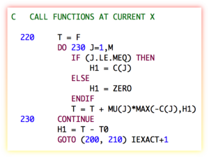
The code is pretty old school and includes numerous obsolescent Fortran features such as arithmetic IF statements, computed and assigned GOTO statements, statement functions, etc. It also includes some non-standard assumptions (implicit saving of variables and initialization to zero).
So, the time is ripe for refactoring SLSQP. Which is what I've done. The refactored version includes some new features and bug fixes, including:
- It is now thread safe. The original version was not thread safe due to the use of saved variables in one of the subroutines.
- It should now be 100% standard compliant (Fortran 2008).
- It now has an easy-to-use object-oriented interface. The
slsqp_class is used for all interactions with the solver. Methods include initialize(), optimize(), and destroy().
- It includes updated versions of some of the third-party routines used in the original code (BLAS, LINPACK, and NNLS).
- It has been translated into free-form source. For this, I used the sample online version of the SPAG Fortran Code Restructuring tool to perform some of the translation, which seemed to work really well. The rest I did manually. Fixed-form source (FORTRAN 77 style) is terrible and needs to die. There's no reason to be using it 25 years after the introduction of free-form source (yes, I'm talking to you Claus 😀).
- The documentation strings in the code have been converted to FORD format, allowing for nicely formatted documentation to be auto-generated (which includes MathJax formatted equations to replace the ASCII ones in the original code). It also generates ultra-slick call graphs like the one below.
- A couple of bug fixes noted elsewhere have been applied (see here and here).
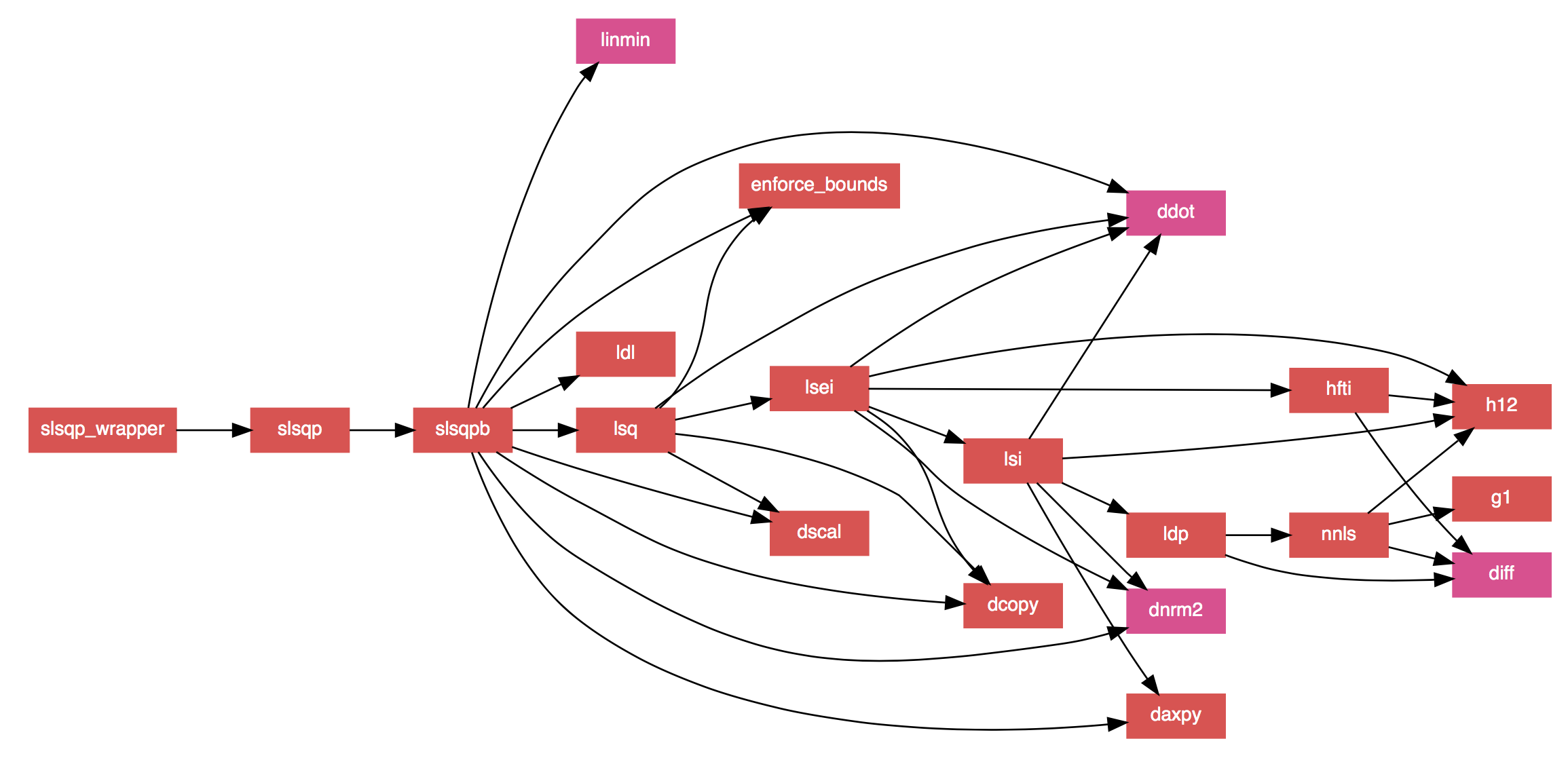
*SLSQP call graph generated by FORD.*
The original code used a "reverse communication" interface, which was one of the workarounds used in old Fortran code to make up for the fact that there wasn't really a good way to pass arbitrary data into a library routine. So, the routine returns after called, requests data, and then is called again. For now, I've kept the reverse communication interface in the core routines (the user never interacts with them directly, however). Eventually, I may do away with this, since I don't think it's particularly useful anymore.
The new code is on GitHub, and is released under a BSD license. There are various additional improvements that could be made, so I'll continue to tinker with it, but for now it seems to work fine. If anyone else finds the new version useful, I'd be interested to hear about it.
See Also
- Dieter Kraft, "A Software Package for Sequential Quadratic Programming", DFVLR-FB 88-28, 1988.
- Dieter Kraft, "Algorithm 733: TOMP–Fortran Modules for Optimal Control Calculations," ACM Transactions on Mathematical Software, Vol. 20, No. 3, p. 262-281 (1994).
Jun 21, 2015
SLSQP [1-2] is a sequential least squares constrained optimization algorithm written by Dieter Kraft in the 1980s. Today, it forms part of the Python pyOpt package for solving nonlinear constrained optimization problems. It was written in FORTRAN 77, and is filled with such ancient horrors like arithmetic IF statements, GOTO statements (even computed and assigned GOTO statements), statement functions, etc. It also assumes the implicit saving of variables in the LINMIN subroutine (which is totally non-standard, but was done by some early compilers), and in some instances assumes that variables are initialized with a zero value (also non-standard, but also done by some compilers). It has an old-fashioned "reverse communication" style interface, with generous use of "WORK" arrays passed around using assumed-size dummy arguments. The pyOpt users don't seem to mind all this, since they are calling it from a Python wrapper, and I guess it works fine (for now).
I don't know if anyone has ever tried to refactor this into modern Fortran with a good object-oriented interface. It seems like it would be a good idea. I've been toying with it for a while. It is always an interesting process to refactor old Fortran code. The fixed-form to free-form conversion can usually be done fairly easily with an automated script, but untangling the spaghetti can be a bit harder. Consider the following code snipet from the subroutine HFTI:
C DETERMINE PSEUDORANK
    DO 90 j=1,ldiag
90  IF(ABS(a(j,j)).LE.tau) GOTO 100
    k=ldiag
    GOTO 110
100 k=j-1
110 kp1=k+1
A modern version that performs the exact same calculation is:
!determine pseudorank:
do j=1,ldiag
    if (abs(a(j,j))<=tau) exit
end do
k=j-1
kp1=j
As you can see, no line numbers or GOTO statements are required. The new version even eliminates one assignment and one addition operation. Note that the refactored version depends on the fact that the index of the DO loop, if it completes the loop (i.e., if the exit statement is not triggered), will have a value of ldiag+1. This behavior has been part of the Fortran standard for some time (perhaps it was not when this routine was written?).
There is also a C translation of SLSQP available, which fixes some of the issues in the original code. Their version of the above code snippet is a pretty straightforward translation of the FORTRAN 77 version, except with all the ugliness of C on full display (a[j + j * a_dim1], seriously?):
/* DETERMINE PSEUDORANK */
i__2 = ldiag;
for (j = 1; j <= i__2; ++j) {
    /* L90: */
    if ((d__1 = a[j + j * a_dim1], fabs(d__1)) <= *tau) {
        goto L100;
    }
}
k = ldiag;
goto L110;
L100:
k = j - 1;
L110:
kp1 = k + 1;
See Also
- Dieter Kraft, "A Software Package for Sequential Quadratic Programming", DFVLR-FB 88-28, 1988.
- Dieter Kraft, "Algorithm 733: TOMP–Fortran Modules for Optimal Control Calculations," ACM Transactions on Mathematical Software, Vol. 20, No. 3, p. 262-281 (1994).
- John Burkardt, LAWSON Least Squares Routines, 21 October 2008. [Fortran 90 versions of the least squares routines used in SLSQP].
Mar 14, 2015
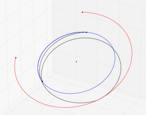
*Earth-Mars Free Return*
Let's try using the Fortran Astrodynamics Toolkit and Pikaia to solve a real-world orbital mechanics problem. In this case, computing the optimal Earth-Mars free return trajectory in the year 2018. This is a trajectory that departs Earth, and then with no subsequent maneuvers, flies by Mars and returns to Earth. The building blocks we need to do this are:
- An ephemeris of the Earth and Mars [DE405]
- A Lambert solver [1]
- Some equations for hyperbolic orbits [given below]
- An optimizer [Pikaia]
The \(\mathbf{v}_{\infty}\) vector of a hyperbolic planetary flyby (using patched conic assumptions) is simply the difference between the spacecraft's heliocentric velocity and the planet's velocity:
- \(\mathbf{v}_{\infty} = \mathbf{v}_{heliocentric} - \mathbf{v}_{planet}\)
The hyperbolic turning angle \(\Delta\) is the angle between \(\mathbf{v}_{\infty}^{-}\) (the \(\mathbf{v}_{\infty}\) before the flyby) and the \(\mathbf{v}_{\infty}^{+}\) (the \(\mathbf{v}_{\infty}\) vector after the flyby). The turning angle can be used to compute the flyby periapsis radius \(r_p\) using the equations:
- \(e = \frac{1}{\sin(\Delta/2)}\)
- \(r_p = \frac{\mu}{v_{\infty}^2}(e-1)\)
So, from the Lambert solver, we can obtain Earth to Mars, and Mars to Earth trajectories (and the heliocentric velocities at each end). These are used to compute the \(\mathbf{v}_{\infty}\) vectors at: Earth departure, Mars flyby (both incoming and outgoing vectors), and Earth return.
There are three optimization variables:
- The epoch of Earth departure [modified Julian date]
- The outbound flight time from Earth to Mars [days]
- The return flyby time from Mars to Earth [days]
There are also two constraints on the heliocentric velocity vectors before and after the flyby at Mars:
- The Mars flyby must be unpowered (i.e., no propulsive maneuver is performed). This means that the magnitude of the incoming (\(\mathbf{v}_{\infty}^-\)) and outgoing (\(\mathbf{v}_{\infty}^+\)) vectors must be equal.
- The periapsis flyby radius (\(r_p\)) must be greater than some minimum value (say, 160 km above the Martian surface).
For the objective function (the quantity that is being minimized), we will use the sum of the Earth departure and return \(\mathbf{v}_{\infty}\) vector magnitudes. To solve this problem using Pikaia, we need to create a fitness function, which is given below:
subroutine obj_func(me,x,f)

!Pikaia fitness function for an Earth-Mars free return

use fortran_astrodynamics_toolkit

implicit none

class(pikaia_class),intent(inout) :: me !pikaia class
real(wp),dimension(:),intent(in) :: x !optimization variable vector
real(wp),intent(out) :: f !fitness value

real(wp),dimension(6) :: rv_earth_0, rv_mars, rv_earth_f
real(wp),dimension(3) :: v1,v2,v3,v4,vinf_0,vinf_f,vinfm,vinfp
real(wp) :: jd_earth_0,jd_mars,jd_earth_f,&
dt_earth_out,dt_earth_return,&
rp_penalty,vinf_penalty,e,delta,rp,vinfmag

real(wp),parameter :: mu_sun = 132712440018.0_wp !sun grav param [km3/s2]
real(wp),parameter :: mu_mars = 42828.0_wp !mars grav param [km3/s2]
real(wp),parameter :: rp_mars_min = 3390.0_wp+160.0_wp !min flyby radius at mars [km]
real(wp),parameter :: vinf_weight = 1000.0_wp !weights for the
real(wp),parameter :: rp_weight = 10.0_wp ! penalty functions

!get times:
jd_earth_0 = mjd_to_jd(x(1)) !julian date of earth departure
dt_earth_out = x(2) !outbound flyby time [days]
dt_earth_return = x(3) !return flyby time [days]
jd_mars = jd_earth_0 + dt_earth_out !julian date of mars flyby
jd_earth_f = jd_mars + dt_earth_return !julian date of earth arrival

!get earth/mars locations (wrt Sun):
call get_state(jd_earth_0,3,11,rv_earth_0) !earth at departure
call get_state(jd_mars, 4,11,rv_mars) !mars at flyby
call get_state(jd_earth_f,3,11,rv_earth_f) !earth at arrival

!compute lambert maneuvers:
call lambert(rv_earth_0,rv_mars, dt_earth_out*day2sec, mu_sun,v1,v2) !outbound
call lambert(rv_mars, rv_earth_f,dt_earth_return*day2sec,mu_sun,v3,v4) !return

!compute v-inf vectors:
vinf_0 = v1 - rv_earth_0(4:6) !earth departure
vinfm = v2 - rv_mars(4:6) !mars flyby (incoming)
vinfp = v3 - rv_mars(4:6) !mars flyby (outgoing)
vinf_f = v4 - rv_earth_f(4:6) !earth return

!the turning angle is the angle between vinf- and vinf+
delta = angle_between_vectors(vinfm,vinfp) !turning angle [rad]
vinfmag = norm2(vinfm) !vinf vector mag (incoming) [km/s]
e = one/sin(delta/two) !eccentricity
rp = mu_mars/(vinfmag*vinfmag)*(e-one) !periapsis radius [km]

!the constraints are added to the fitness function as penalties:
if (rp>=rp_mars_min) then
    rp_penalty = zero !not active
else
    rp_penalty = rp_mars_min - rp
end if
vinf_penalty = abs(norm2(vinfm) - norm2(vinfp))

!fitness function (to maximize):
f = - ( norm2(vinf_0) + &
    norm2(vinf_f) + &
    vinf_weight*vinf_penalty + &
    rp_weight*rp_penalty )

end subroutine obj_func
The lambert routine called here is simply a wrapper to solve_lambert_gooding that computes both the "short way" and "long way" transfers, and returns the one with the lowest total \(\Delta v\). The two constraints are added to the objective function as penalties (to be driven to zero). Pikaia is then initialized and called by:
program flyby

use pikaia_module
use fortran_astrodynamics_toolkit

implicit none

integer,parameter :: n = 3

type(pikaia_class) :: p
real(wp),dimension(n) :: x,xl,xu
integer :: status,iseed
real(wp) :: f

!set random number seed:
iseed = 371

!bounds:
xl = [jd_to_mjd(julian_date(2018,1,1,0,0,0)), 100.0_wp,100.0_wp]
xu = [jd_to_mjd(julian_date(2018,12,31,0,0,0)),400.0_wp,400.0_wp]

call p%init(n,xl,xu,obj_func,status,&
            ngen = 1000, &
            np = 200, &
            nd = 9, &
            ivrb = 0, &
            convergence_tol = 1.0e-6_wp, &
            convergence_window = 200, &
            initial_guess_frac = 0.0_wp, &
            iseed = iseed )

call p%solve(x,f,status)

end program flyby
The three optimization variables are bounded: the Earth departure epoch must occur sometime in 2018, and the outbound and return flight times must each be between 100 and 400 days.
Running this program, we can get different solutions (depending on the value set for the random seed, and also the Pikaia settings). The best one I've managed to get with minimal tweaking is this:
- Earth departure epoch: MJD 58120 (Jan 2, 2018)
- Outbound flight time: 229 days
- Return flight time: 271 days
Which is similar to the solution shown in [2].
References
- R.H. Gooding, "A procedure for the solution of Lambert's orbital boundary-value problem", Celestial Mechanics and Dynamical Astronomy, Vol. 48, No. 2, 1990.
- Dennis Tito's 2021 Human Mars Flyby Mission Explained. SPACE.com, February 27, 2014.
- J.E. Prussing, B.A. Conway, "Orbital Mechanics", Oxford University Press, 1993.
Mar 09, 2015

I've started a new project on Github for a new modern object-oriented version of the Pikaia genetic algorithm code. This is a refactoring and upgrade of the Pikaia code from the High Altitude Observatory. The original code is public domain and was written by Paul Charbonneau & Barry Knapp (version 1.2 was released in 2003). The new code differs from the old code in the following respects:
- The original fixed-form source (FORTRAN 77) was converted to free-form source.
- The code is now object-oriented Fortran 2003/2008. All user interaction is now through a class, which is the only public entity in the module.
- All real variables are now 8 bytes (a.k.a. "double precision"). The precision can also be changed by the user by modifying the
wp parameter.
- The random number generator was replaced with calls to the intrinsic Fortran
random_number function.
- There are various new options (e.g., a convergence window with a tolerance can be specified as a stopping condition, and the user can specify a subroutine for reporting the best solution at each generation).
- Mapping the variables to be between 0 and 1 now occurs internally, rather than requiring the user to do it.
- Can now include an initial guess in the initial population.
This is another example of how older Fortran codes can be refactored to bring them up to date with modern computing concepts without doing that much work. In my opinion, the object-oriented Fortran 2003 interface is a lot better than the old FORTRAN 77 version. For one, it's easier to follow. Also, data can now easily be passed into the user fitness function by extending the pikaia class and putting the data there. No common blocks necessary!
References
- Original Pikaia code and documentation [High Altitude Observatory]