Oct 18, 2019

Just in case you find yourself needing to do some multidimensional data interpolation with modern Fortran:
- I just published a modernized version of REGRIDPACK, a library for "regriding" 1D-4D data sets using linear and spline interpolation. The original version of this library (which used to be called TLCPACK) was formerly available from the UCAR website, but it is now nowhere to be seen. It was a well-written library, and had the nice feature of being able to specify linear or spline interpolation independently for each dimension. My refactoring is simply an update of the old code to modern standards.
- I also recently added nearest neighbor interpolation to my Finterp library. So, now you can perform linear and nearest neighbor interpolation/extrapolation on 1D-6D data sets.
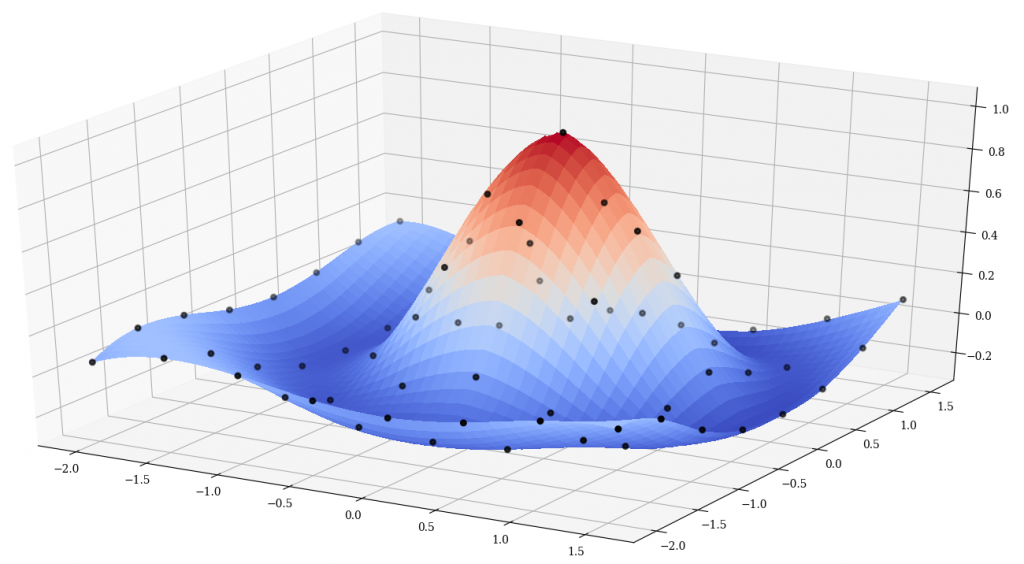
- My Bspline-Fortran library can also be used for interpolation/extrapolation of 1D-6D data sets using B-splines. This library is being used by several people for CFD work, it seems.
There are precious few modern Fortran libraries for other types of interpolation. Here are a couple:
- FOLLIA -- Fortran Library for Lagrange Interpolation
- curvefit -- A library for fitting functions to sets of data.
There are also any number of old school FORTRAN 77 codes out there that haven't been updated in decades, but still work fine for what they do, including:
- PCHIP -- Piecewise Cubic Hermite Interpolation Package from SLATEC.
- PPPACK -- Piecewise polynomial interpolation code from from A Practical Guide to Splines by C. de Boor.
- FITPACK -- a collection of FORTRAN programs for curve and surface fitting with splines and tensor product splines.
See also
Mar 05, 2017
I just released some updates to my two most popular Fortran libraries on GitHub: JSON-Fortran and bspline-fortran. Coincidently, both are now at v5.2.0. Details of the updates are:
JSON-Fortran

There are several new features in this release. The biggest update is that now the code can parse JSON files that include comments (it just ignores them). You can even specify the character that identifies a comment. For example, if using # as a comment character, the following file can now be parsed just fine:
{
    "t": 0.12345,  # this is the time
    "x": 123.7173  # this is the state
}
Technically, comments are not part of the JSON standard. Douglas Crockford, the creator of JSON, had his reasons [1] for not including them, which I admit I don't understand (something about parsing directives and interoperability?) I mainly use JSON for configuration files, where it is nice to have comments. Crockford's suggestion for this use case is to pipe your commented JSON files through something called JSMin before parsing, a solution which seems somewhat ridiculous for Fortran users. So, never fear, now we can have comments in our JSON files and continue not using JavaScript for anything.
Another big change is the addition of support for the RFC 6901 "JSON Pointer" path specification [2]. This can be used to retrieve data from a JSON structure using its path. Formerly, JSON-Fortran used a simple path specification syntax, which broke down if the keys contained special characters such as ( or ). The new way works for all keys.
Bspline-Fortran

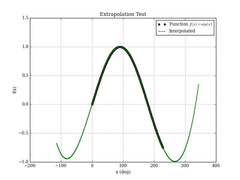
A minor update to Bspline-Fortran is the addition of an extrapolation mode. Formerly, if an interpolation was requested outside the bounds of the data, an error was returned. Now, the user has the option of enabling extrapolation.
See also
- D. Crockford, "Comments in JSON", Apr 30, 2012 [Google Plus]
- JavaScript Object Notation (JSON) Pointer, RFC 6901, April 2013 [IETF]
Dec 12, 2016
In an earlier post, I mentioned that we needed an object-oriented modern Fortran library for multidimensional linear interpolation. Well, here it is. I call it finterp, and it is available on GitHub. It can be used for 1D-6D interpolation/extrapolation of data on a regular grid (i.e., not scattered). It has a similar object-oriented interface as my bspline-fortran library, with initialize, evaluate, and destroy methods like so:
type(linear_interp_3d) :: interp
call interp%initialize(xvec,yvec,zvec,fmat,iflag)
call interp%evaluate(x,y,z,f)
call interp%destroy()
For example, the low-level 3D interpolation evaluate routine is:
pure subroutine interp_3d(me,x,y,z,fxyz)

implicit none

class(linear_interp_3d),intent(inout) :: me
real(wp),intent(in) :: x
real(wp),intent(in) :: y
real(wp),intent(in) :: z
real(wp),intent(out) :: fxyz !! Interpolated ( f(x,y,z) )

integer,dimension(2) :: ix, iy, iz
real(wp) :: p1, p2, p3
real(wp) :: q1, q2, q3
integer :: mflag
real(wp) :: fx11, fx21, fx12, fx22, fxy1, fxy2

call dintrv(me%x,x,me%ilox,ix(1),ix(2),mflag)
call dintrv(me%y,y,me%iloy,iy(1),iy(2),mflag)
call dintrv(me%z,z,me%iloz,iz(1),iz(2),mflag)

q1 = (x-me%x(ix(1)))/(me%x(ix(2))-me%x(ix(1)))
q2 = (y-me%y(iy(1)))/(me%y(iy(2))-me%y(iy(1)))
q3 = (z-me%z(iz(1)))/(me%z(iz(2))-me%z(iz(1)))
p1 = one-q1
p2 = one-q2
p3 = one-q3

fx11 = p1*me%f(ix(1),iy(1),iz(1)) + q1*me%f(ix(2),iy(1),iz(1))
fx21 = p1*me%f(ix(1),iy(2),iz(1)) + q1*me%f(ix(2),iy(2),iz(1))
fx12 = p1*me%f(ix(1),iy(1),iz(2)) + q1*me%f(ix(2),iy(1),iz(2))
fx22 = p1*me%f(ix(1),iy(2),iz(2)) + q1*me%f(ix(2),iy(2),iz(2))
fxy1 = p2*( fx11 ) + q2*( fx21 )
fxy2 = p2*( fx12 ) + q2*( fx22 )

fxyz = p3*( fxy1 ) + q3*( fxy2 )

end subroutine interp_3d
The finterp library is released under a permissive BSD-3 license. As far as I can tell, it is unique among publicly-available Fortran codes in providing linear interpolation for up to 6D data sets. There used to be a Fortran 77 library called REGRIDPACK for regridding 1D-4D data sets (it had the option to use linear or cubic interpolation independently for each dimension). Written by John C. Adams at the National Center for Atmospheric Research in 1999, it used to be hosted at the UCAR website, but the link is now dead. You can still find it on the internet though, as part of other projects (for example here, where it is being used via a Python wrapper). But the licensing is unclear to me.
The dearth of easy-to-find, easy-to-use, high-quality open source modern Fortran libraries is a big problem for the long-term future of the language. Fortran users don't seem to be as interested in promoting their language as users of some of the newer programming languages are. There is a group of us working to change this, but we've got a long way to go. For example, Julia, a programming language only four years old, already has a ton of libraries, some of which are just wrappers to Fortran 77 code that no one's ever bothered to modernize. They even have a yearly conference. An in depth article about this state of affairs is a post for another day.
References
Feb 28, 2016
Some years ago, I needed a Fortran routine to do linear interpolation of a multidimensional (up to 6D) data set. Not wanting to reinvent the wheel, I ended up using a routine called FINT from CERNLIB (documentation here). It is written in Fortran 66, and has some hard-coded limits on the number of dimensions that can be used, but these are not fundamental to the algorithm. With a few minor changes, the routine can be used for interpolation of any number of dimensions. I present below a modern Fortran version that removes the limitations. Note that the original code is GPL licensed, thus so is this modification.
function fint(narg,arg,nent,ent,table)

use iso_fortran_env, only: wp => real64

implicit none

real(wp) :: fint
integer,intent(in) :: narg
integer,dimension(narg),intent(in) :: nent
real(wp),dimension(narg),intent(in) :: arg
real(wp),dimension(:),intent(in) :: ent
real(wp),dimension(:),intent(in) :: table

integer,dimension(2**narg) :: index
real(wp),dimension(2**narg) :: weight
logical :: mflag,rflag
real(wp) :: eta,h,x
integer :: i,ishift,istep,k,knots,lgfile,&
           lmax,lmin,loca,locb,locc,ndim

!some error checks:
if (size(ent)/=sum(nent)) &
    error stop 'size of ent is incorrect.'
if (size(table)/=product(nent)) &
    error stop 'size of table is incorrect.'
if (narg<1) &
    error stop 'invalid value of narg.'

lmax = 0
istep = 1
knots = 1
index(1) = 1
weight(1) = 1.0_wp

main: do i = 1 , narg
    x = arg(i)
    ndim = nent(i)
    loca = lmax
    lmin = lmax + 1
    lmax = lmax + ndim
    if ( ndim>2 ) then
        locb = lmax + 1
        do
            locc = (loca+locb)/2
            if ( x<ent(locc) ) then
                locb = locc
            else if ( x==ent(locc) ) then
                ishift = (locc-lmin)*istep
                do k = 1 , knots
                    index(k) = index(k) + ishift
                end do
                istep = istep*ndim
                cycle main
                else
                loca = locc
            end if
            if ( locb-loca<=1 ) exit
        end do
        loca = min(max(loca,lmin),lmax-1)
        ishift = (loca-lmin)*istep
        eta = (x-ent(loca))/(ent(loca+1)-ent(loca))
    else
        if ( ndim==1 ) cycle main
        h = x - ent(lmin)
        if ( h==0.0_wp ) then
            istep = istep*ndim
            cycle main
        end if
        ishift = istep
        if ( x-ent(lmin+1)==0.0_wp ) then
            do k = 1 , knots
                index(k) = index(k) + ishift
            end do
            istep = istep*ndim
            cycle main
        end if
        ishift = 0
        eta = h/(ent(lmin+1)-ent(lmin))
    end if
    do k = 1 , knots
        index(k) = index(k) + ishift
        index(k+knots) = index(k) + istep
        weight(k+knots) = weight(k)*eta
        weight(k) = weight(k) - weight(k+knots)
    end do
    knots = 2*knots
    istep = istep*ndim
end do main

fint = 0.0_wp
do k = 1 , knots
    i = index(k)
    fint = fint + weight(k)*table(i)
end do

end function fint
As I recall, I wrote wrappers to this function in order to be able to input the data in a more reasonable format. For example, for a five dimensional data set it is more natural to input the five rank-1 abscissa vectors and the rank-5 ordinate matrix. The disadvantage of this routine is that you have to stuff the ordinate matrix into a vector (as well as stuffing all the abscissa vectors into a single vector). This could also be an advantage in some cases, since Fortran arrays have a maximum rank. For Fortran 90, it was 7, while Fortran 2008 expanded this to 15 (the current Intel Fortran Compiler allows up to 31 as a non-standard extension). If you ever, for example, needed to interpolate 32-dimensional data (assuming you had enough RAM), you could do it with FINT without having to declare any rank-32 matrices. In any event, an example 5D wrapper for FINT is given here:
function fint_5d_wrapper(x,y,z,q,r,&
                         xvec,yvec,zvec,qvec,&
                         rvec,fmat) result(f)

use iso_fortran_env, only: wp => real64

implicit none

integer,parameter :: narg = 5

real(wp) :: f
real(wp),intent(in) :: x,y,z,q,r
real(wp),dimension(:),intent(in) :: xvec
real(wp),dimension(:),intent(in) :: yvec
real(wp),dimension(:),intent(in) :: zvec
real(wp),dimension(:),intent(in) :: qvec
real(wp),dimension(:),intent(in) :: rvec
real(wp),dimension(:,:,:,:,:),intent(in) :: fmat

integer,dimension(narg) :: nent

nent(1) = size(xvec)
nent(2) = size(yvec)
nent(3) = size(zvec)
nent(4) = size(qvec)
nent(5) = size(rvec)

f = fint(narg,[x,y,z,q,r],nent,&
    [xvec,yvec,zvec,qvec,rvec],&
    reshape(fmat,[product(nent)]))

end function fint_5d_wrapper
This works well enough, but note that it isn't very computationally efficient since we are creating temporary copies of the potentially large data arrays (including having to reshape a rank-5 matrix) every time we do an interpolation. While the logic of FINT is a bit hard to fathom, the actual equations are fairly simple (see here, for example). What we really need now is an object-oriented modern Fortran library for multidimensional linear interpolation. Stay tuned...
References
Nov 06, 2015

My bspline-fortran multidimensional interpolation library is now at version 4.0. The documentation can be found here. Since I first mentioned it here, I've made many updates to this library, including:
- Added object-oriented wrappers to the core routines. The user now has the choice to use the older subroutine interface or the new object-oriented interface.
- Added a set of 1D routines (suggested by a user on GitHub). The library now works for 1D-6D data sets.
- Everything is now thread-safe for your multithreaded pleasure.
The new object-oriented interface makes it pretty easy to use from modern Fortran. The classes have only three methods (initialize, evaluate, and destroy). For example, a 3D case would look like this:
type(bspline_3d) :: s
call s%initialize(x,y,z,fcn,kx,ky,kz,iflag)
call s%evaluate(xval,yval,zval,idx,idy,idz,f,iflag)
call s%destroy()
The core routines of bspline-fortran were written in the early 1980s. Good Fortran code can live on for decades after it is written. While this is great, it also means that there is a lot of old Fortran code out there that is written in a coding style that no modern programmer should accept. This can be OK for well documented library routines that the user never needs to change (see, for example SPICE or LAPACK). However, refactoring old code using modern concepts can provide many advantages, as is demonstrated in this case.
See also
- DBSPLIN and DTENSBS from the NIST Core Math Library.
- Carl de Boor, A Practical Guide to Splines, Springer-Verlag, New York, 1978.
Apr 11, 2015
A simple Fortran implementation of interpolation by Lagrange polynomials is given below. Though named after Joseph-Louis Lagrange, the formula was first discovered by English mathematician Edward Waring.
subroutine lagrange_interpolation(xx,yy,x,y)
!
! Interpolate xx=[x1,x2,...xn]
! yy=[f(x1),f(x2),...,f(xn)]
! Using Lagrange polynomial P(x)
! Returns y = P(x)
!
use,intrinsic :: iso_fortran_env, wp => real64

implicit none

real(wp),dimension(:),intent(in) :: xx
real(wp),dimension(:),intent(in) :: yy
real(wp),intent(in) :: x
real(wp),intent(out) :: y

!local variables:
integer :: j,k,n,m
real(wp) :: p

!check number of points:
n = size(xx)
m = size(yy)
if (n/=m) error stop &
    'Error: vectors must be the same size.'

!sum each of the Pj(x) terms:
y = 0.0_wp
do j=1,n
    !compute Pj(x):
    p = yy(j)
    do k=1,n
        if (k/=j) p = p * (x-xx(k)) / (xx(j)-xx(k))
    end do
    y = y + p
end do

end subroutine lagrange_interpolation
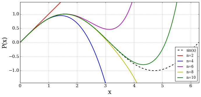
Examples of interpolating polynomials for the \(\sin(x)\) function are shown here for different numbers of points \(x=[0.0, 0.01]\), \(x=[0.0, 0.01, 0.02]\), etc.

References
Feb 25, 2015
I just started a new modern Fortran software library called bspline-fortran, which is for multidimensional (multivariate) b-spline interpolation of data defined on a regular grid. It is available on GitHub, and released under a permissive BSD-style license.
It seems impossible to find code for higher than 3D spline interpolation on the internet. Einspline only has 1D-3D, as do the NIST Core Math Library DBSPLIN and DTENSBS routines. Python's SciPy stops at 2D (Bivariate splines). At first glance, the SciPy routine map_coordinates seems to do what I want, but not really since there doesn't seem to be any way to specify the abscissa vectors (x, y, z, etc.). Note: maybe there is a way, but looking at the less-than-great documentation, the minimally-commented C code, and then reading several confusing Stack Overflow posts didn't help me much. Apparently, I'm not the only one confused by this routine.
After much searching, I finally just took the 2D and 3D NIST routines (written in 1982), refactored them significantly so I could better understand what they were doing, and then extended the algorithm into higher dimensions (which is actually quite easy to do for b-splines). The original FORTRAN 77 code was somewhat hard to follow, since it was stuffing matrices into a giant WORK vector, which required a lot of obscure bookkeeping of indices. For example, I replaced this bit of code:
    IZM1 = IZ - 1
    KCOLY = LEFTY - KY + 1
    DO 60 K=1,KZ
      I = (K-1)*KY + 1
      J = IZM1 + K
      WORK(J) = DBVALU(TY(KCOLY),WORK(I),KY,KY,IDY,YVAL,INBV1,WORK(IW))
60  CONTINUE
with this:
kcoly = lefty - ky + 1
do k=1,kz
    temp2(k) = dbvalu(ty(kcoly:),temp1(:,k),ky,ky,idy,yval,inbv1,work)
end do
which makes it a lot easier to deal with and add the extra dimensions as necessary.
The new library contains routines for 2D, 3D, 4D, 5D, and 6D interpolation. It seems like someone else may find them useful, I don't know why they don't seem to be available anywhere else. Eventually, I'll add object-oriented wrappers for the core routines, to make them easier to use.
