
The rocket equation describes the basic principles of a rocket in the absence of external forces. Various forms of this equation relate the following fundamental parameters:
- the engine thrust (\(T\)),
- the engine specific impulse (\(I_{sp}\)),
- the engine exhaust velocity (\(c\)),
- the initial mass (\(m_i\)),
- the final mass (\(m_f\)),
- the burn duration (\(\Delta t\)), and
- the effective delta-v (\(\Delta v\)) of the maneuver.
The rocket equation is:
- \(\Delta v = c \ln \left( \frac{m_i}{m_f} \right)\)
The engine specific impulse is related to the engine exhaust velocity by: \(c = I_{sp} g_0\), where \(g_0\) is the standard Earth gravitational acceleration at sea level (defined to be exactly 9.80665 \(m/s^2\)). The thrust is related to the mass flow rate (\(\dot{m}\)) of the engine by: \(T = c \dot{m}\). This can be used to compute the duration of the maneuver as a function of the \(\Delta v\):
- \(\Delta t = \frac{c m_i}{T} \left( 1 - e^{-\frac{\Delta v}{c}} \right)\)
A Fortran module implementing these equations is given below.
module rocket_equation

use,intrinsic :: iso_fortran_env, only: wp => real64

implicit none

!two ways to compute effective delta-v
interface effective_delta_v
procedure :: effective_dv_1,effective_dv_2
end interface effective_delta_v

real(wp),parameter,public :: g0 = 9.80665_wp ![m/s^2]

contains

pure function effective_dv_1(c,mi,mf) result(dv)

real(wp) :: dv ! effective delta v [m/s]
real(wp),intent(in) :: c ! exhaust velocity [m/s]
real(wp),intent(in) :: mi ! initial mass [kg]
real(wp),intent(in) :: mf ! final mass [kg]

dv = c*log(mi/mf)

end function effective_dv_1

pure function effective_dv_2(c,mi,T,dt) result(dv)

real(wp) :: dv ! delta-v [m/s]
real(wp),intent(in) :: c ! exhaust velocity [m/s]
real(wp),intent(in) :: mi ! initial mass [kg]
real(wp),intent(in) :: T ! thrust [N]
real(wp),intent(in) :: dt ! duration of burn [sec]

dv = -c*log(1.0_wp-(T*dt)/(c*mi))

end function effective_dv_2

pure function burn_duration(c,mi,T,dv) result(dt)

real(wp) :: dt ! burn duration [sec]
real(wp),intent(in) :: c ! exhaust velocity [m/s]
real(wp),intent(in) :: mi ! initial mass [kg]
real(wp),intent(in) :: T ! engine thrust [N]
real(wp),intent(in) :: dv ! delta-v [m/s]

dt = (c*mi)/T*(1.0_wp-exp(-dv/c))

end function burn_duration

pure function final_mass(c,mi,dv) result(mf)

real(wp) :: mf ! final mass [kg]
real(wp),intent(in) :: c ! exhaust velocity [m/s]
real(wp),intent(in) :: mi ! initial mass [kg]
real(wp),intent(in) :: dv ! delta-v [m/s]

mf = mi/exp(dv/c)

end function final_mass

end module rocket_equation
References
- J.E. Prussing, B.A. Conway, "Orbital Mechanics", Oxford University Press, 1993.

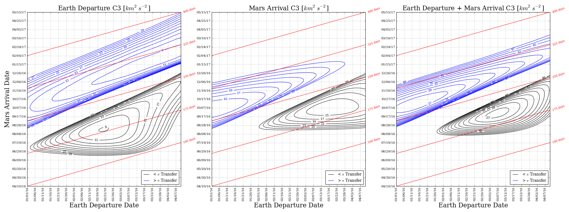
A porkchop plot is a data visualization tool used in interplanetary mission design which displays contours of various quantities as a function of departure and arrival date. Example pork chop plots for 2016 Earth-Mars transfers are shown here. The x-axis is the Earth departure date, and the y-axis is the Mars arrival date. The contours show the Earth departure C3, the Mars arrival C3, and the sum of the two. C3 is the "characteristic energy" of the departure or arrival, and is equal to the \(v_{\infty}^2\) of the hyperbolic trajectory. Each point on the curve represents a ballistic Earth-Mars transfer (computed using a Lambert solver). The two distinct black and blue contours on each plot represent the "short way" (\(<\pi\)) and "long way" (\(>\pi\)) transfers. The contours look vaguely like pork chops, the centers being the lowest C3 value, and thus optimal transfers. The January - October 2016 opportunity will be used for the ExoMars Trace Gas Orbiter, and the March - September 2016 opportunity will be used for InSight.
References
- A. B. Sergeyevsky, G. C. Snyder, R. A. Cunniff, "Interplanetary Mission Design Handbook, Volume I, Part 2: Earth to Mars Ballistic Mission Opportunities, 1990-2005", NASA JPL, September 1983.
- L. M. Burke, R. D. Falck, and M. L. McGuire, "Interplanetary Mission Design Handbook: Earth-to-Mars Mission Opportunities 2026 to 2045", NASA/TM—2010-216764, October 2010.
- Chauncey Uphoff, The History of the Term C3, 2001.
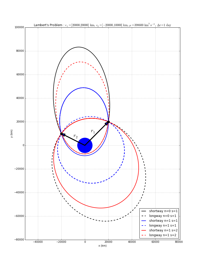
Lambert's problem is to solve for the orbit transfer that connects two position vectors in a given time of flight. It is one of the basic problems of orbital mechanics, and was solved by Swiss mathematician Johann Heinrich Lambert.
A standard Fortran 77 implementation of Lambert's problem was presented by Gooding [1]. A modern update to this implementation is included in the Fortran Astrodynamics Toolkit, which also includes a newer algorithm from Izzo [2].
There can be multiple solutions to Lambert's problem, which are classified by:
- Direction of travel (i.e., a "short" way or "long" way transfer).
- Number of complete revolutions (N=0,1,...). For longer flight times, solutions exist for larger values of N.
- Solution number (S=1 or S=2). The multi-rev cases can have two solutions each.
In the example shown here, there are 6 possible solutions:
References
- R.H, Gooding. "A procedure for the solution of Lambert's orbital boundary-value problem", Celestial Mechanics and Dynamical Astronomy, Vol. 48, No. 2, 1990.
- D. Izzo, "Revisiting Lambert’s problem", Celestial Mechanics and Dynamical Astronomy, Oct. 2014.
Fortran 2003 was a significant update to Fortran 95 (probably something on the order of the update from C to C++). It brought Fortran into the modern computing world with the addition of object oriented programming features such as type extension and inheritance, polymorphism, dynamic type allocation, and type-bound procedures.
The following example shows an implementation of an object oriented class to perform numerical integration of a user-defined function using a Runge-Kutta method (in this case RK4). First, an abstract rk_class is defined, which is then extended to create the RK4 class by associating the deferred step method to rk4. Other RK classes could also be created in a similar manner. In order to use the class, it is only necessary to set n (the number of variables in the state vector) and f (the user-supplied derivative function), and then call the integrate method.
module rk_module

use, intrinsic :: iso_fortran_env, wp => real64 !double precision reals

implicit none

real(wp),parameter :: zero = 0.0_wp

!main integration class:
type,abstract,public :: rk_class
    private
    !user specified number of variables:
    integer :: n = 0
    !user-specified derivative function:
    procedure(deriv_func),pointer :: f => null()
    contains
    procedure,non_overridable,public :: integrate !main integration routine
    procedure(step_func),deferred :: step !the step routine for the selected method
end type rk_class

!extend the abstract class to create an RK4 method:
! [all we need to do is set the step function]
type,extends(rk_class),public :: rk4_class
    contains
    procedure :: step => rk4
end type rk4_class

interface

    subroutine deriv_func(me,t,x,xdot) !derivative function
    import :: rk_class,wp
    implicit none
    class(rk_class),intent(inout) :: me
    real(wp),intent(in) :: t
    real(wp),dimension(me%n),intent(in) :: x
    real(wp),dimension(me%n),intent(out) :: xdot
    end subroutine deriv_func

    subroutine step_func(me,t,x,h,xf) !rk step function
    import :: rk_class,wp
    implicit none
    class(rk_class),intent(inout) :: me
    real(wp),intent(in) :: t
    real(wp),dimension(me%n),intent(in) :: x
    real(wp),intent(in) :: h
    real(wp),dimension(me%n),intent(out) :: xf
    end subroutine step_func

end interface

contains

subroutine integrate(me,t0,x0,h,tf,xf)
! main integration routine

implicit none

class(rk_class),intent(inout) :: me
real(wp),intent(in) :: t0
real(wp),dimension(me%n),intent(in) :: x0
real(wp),intent(in) :: h
real(wp),intent(in) :: tf
real(wp),dimension(me%n),intent(out) :: xf

real(wp) :: t,dt,t2
real(wp),dimension(me%n) :: x
logical :: last

if (h==zero) then
    xf = x0
else

    t = t0
    x = x0
    dt = h
    do
        t2 = t + dt
        last = ((dt>=zero .and. t2>=tf) .or. & !adjust last time step
               (dt<zero .and. t2<=tf))         !
        if (last) dt = tf-t                    !
        call me%step(t,x,dt,xf)
        if (last) exit
        x = xf
        t = t2
    end do

end if

end subroutine integrate

subroutine rk4(me,t,x,h,xf)
! Take one Runge Kutta 4 integration step: t -> t+h (x -> xf)

implicit none

class(rk4_class),intent(inout) :: me
real(wp),intent(in) :: t
real(wp),dimension(me%n),intent(in) :: x
real(wp),intent(in) :: h
real(wp),dimension(me%n),intent(out) :: xf

!local variables:
real(wp),dimension(me%n) :: f1,f2,f3,f4
real(wp) :: h2

!parameters:
real(wp),parameter :: half = 0.5_wp
real(wp),parameter :: six = 6.0_wp

h2 = half*h

call me%f(t,x,f1)
call me%f(t+h2,x+h2*f1,f2)
call me%f(t+h2,x+h2*f2,f3)
call me%f(t+h,x+h*f3,f4)

xf = x + h*(f1+f2+f2+f3+f3+f4)/six

end subroutine rk4

end module rk_module
An example use of this module follows. Here, we are integrating the equations of motion of a spacecraft in Earth orbit, using two-body assumptions: \(\ddot{\mathbf{r}} = -\frac{\mu}{r^3}\mathbf{r}\)
The rk4_class is extended to create a new spacecraft class, which contains the data required by the derivative routine (in this case, simply the central body gravitational parameter mu). A more complicated version could also include spherical harmonic gravity, solar radiation pressure, atmospheric drag, engine thrust, etc. Note that the select type statement is necessary in the derivative routine in order to access the data from the extended type.
program main

use rk_module

!spacecraft propagation type:
! extend the rk class to include data used in the deriv routine
type,extends(rk4_class) :: spacecraft
    real(wp) :: mu = zero ! central body gravitational
                          ! parameter (km^3/s^2)
end type spacecraft

integer,parameter :: n=6 !number of state variables
type(spacecraft) :: s
real(wp) :: t0,tf,x0(n),dt,xf(n)

!constructor:
s = spacecraft(n=n,f=twobody,mu=398600.436233_wp) !main body is Earth

!initial conditions:
x0 = [10000.0_wp,10000.0_wp,10000.0_wp,& !initial state [x,y,z] (km)
      1.0_wp,2.0_wp,3.0_wp]              !              [vx,vy,yz] (km/s)
t0 = zero !initial time (sec)
dt = 10.0_wp !time step (sec)
tf = 1000.0_wp !final time (sec)

call s%integrate(t0,x0,dt,tf,xf)
write(*,'(A/,*(F15.6/))') 'Final state:',xf

contains

subroutine twobody(me,t,x,xdot)
! derivative routine for two-body orbit propagation

implicit none

class(rk_class),intent(inout) :: me
real(wp),intent(in) :: t
real(wp),dimension(me%n),intent(in) :: x
real(wp),dimension(me%n),intent(out) :: xdot

real(wp),dimension(3) :: r,v,a_grav
real(wp) :: rmag

select type (me)
class is (spacecraft)

    r = x(1:3)
    v = x(4:6)
    rmag = norm2(r)
    a_grav = -me%mu/rmag**3 * r !accel. due to gravity

    xdot(1:3) = v
    xdot(4:6) = a_grav

end select

end subroutine twobody

end program main
The result is:
Final state: 10667.963305 11658.055962 12648.148619 0.377639 1.350074 2.322509
See also
- Object-Oriented Programming in Fortran 2003 Part 1: Code Reusability, PGI Insider, Feb. 2011.
- Object-Oriented Programming in Fortran 2003 Part 2: Data Polymorphism, PGI Insider, June 2011.
- Fortran Astrodynamics Toolkit (Github)
JPL just released a new version of the SPICE Toolkit (N65). According to the What's New page, changes include:
- support for some new environments and termination of some old environments
- new Geometry Finder (GF) interfaces -- illumination angle search, phase angle search, user-defined binary quantity search
- new high-level SPK APIs allowing one to specify the observer or target as a location with a constant position and velocity rather than as an ephemeris object
- new high-level APIs that check for occultation and in-Field-Of-View (FOV) conditions
- new high-level illumination angle routines
- new high-level reference frame transformation routine
- new high-level coordinate system transformation routine for states
- many Icy and Mice APIs that were formerly available only in SPICELIB and CSPICE
- new data types: SPK (19, 20, 21), PCK (20), and CK (6)
- performance improvements in the range of 10-50 percent for some types of use
- ability to load up to 5000 kernels
- increased buffers in the POOL and in SPK and CK segment search subsystems
- new built-in body name/ID code mappings and body-fixed reference frames
- a significant upgrade of utility SPKDIFF including the ability to sample SPK data
- updates to other toolkit utilities -- BRIEF, CKBRIEF, FRMDIFF, MKSPK, MSOPCK
- bug fixes in Toolkit and utility programs
I'm starting a new project on GitHub: the Fortran Astrodynamics Toolkit. Hardly anyone is developing open source orbital mechanics software for modern Fortran, so the time has come. Most of the code from this blog will eventually find its way there. My goal is to include modern Fortran implementations of all the standard orbital mechanics algorithms such as:
- Lambert solvers
- Kepler propagators
- ODE solvers (Runge-Kutta, Nyström, Adams)
- Orbital element conversions
Then we'll see where it goes from there. The code will be released under a permissive BSD style license.