Degenerate Conic

IAU Rotation Models

The IAU Working Group on Cartographic Coordinates and Rotational Elements (WGCCRE) is the keeper of official models that describe the cartographic coordinates and rotational elements of planetary bodies (such as the Earth, satellites, minor planets, and comets). Periodically, they release a report containing the coefficients to compute body orientations, based on the latest data available. These coefficients allow one to compute the rotation matrix from the ICRF frame to a body-fixed frame (for example, IAU Earth) by giving the direction of the pole vector and the prime meridian location as functions of time. An example Fortran module illustrating this for the IAU Earth frame is given below. The coefficients are taken from the 2009 IAU report [Reference 1]. Note that the IAU models are also available in SPICE (as "IAU_EARTH", "IAU_MOON", etc.). For Earth, the IAU model is not suitable for use in applications that require the highest possible accuracy (for that a more complex model would be necessary), but is quite acceptable for many applications.

module iau_orientation_module

use, intrinsic :: iso_fortran_env, only: wp => real64

implicit none

private

!constants:
real(wp),parameter :: zero = 0.0_wp
real(wp),parameter :: one = 1.0_wp
real(wp),parameter :: pi = acos(-one)
real(wp),parameter :: pi2 = pi/2.0_wp
real(wp),parameter :: deg2rad = pi/180.0_wp
real(wp),parameter :: sec2day = one/86400.0_wp
real(wp),parameter :: sec2century = one/3155760000.0_wp

public :: icrf_to_iau_earth

contains

!Rotation matrix from ICRF to IAU_EARTH
pure function icrf_to_iau_earth(et) result(rotmat)

implicit none

real(wp),intent(in) :: et !ephemeris time [sec from J2000]
real(wp),dimension(3,3) :: rotmat !rotation matrix

real(wp) :: w,dec,ra,d,t
real(wp),dimension(3,3) :: tmp

d = et * sec2day !days from J2000
t = et * sec2century !Julian centuries from J2000

ra = ( - 0.641_wp * t ) * deg2rad
dec = ( 90.0_wp - 0.557_wp * t ) * deg2rad
w = ( 190.147_wp + 360.9856235_wp * d ) * deg2rad

!it is a 3-1-3 rotation:
tmp = matmul( rotmat_x(pi2-dec), rotmat_z(pi2+ra) )
rotmat = matmul( rotmat_z(w), tmp )

end function icrf_to_iau_earth

!The 3x3 rotation matrix for a rotation about the x-axis.
pure function rotmat_x(angle) result(rotmat)

implicit none

real(wp),dimension(3,3) :: rotmat !rotation matrix
real(wp),intent(in) :: angle !angle [rad]

real(wp) :: c,s

c = cos(angle)
s = sin(angle)

rotmat = reshape([one, zero, zero, &
                  zero, c, -s, &
                  zero, s, c],[3,3])

end function rotmat_x

!The 3x3 rotation matrix for a rotation about the z-axis.
pure function rotmat_z(angle) result(rotmat)

implicit none

real(wp),dimension(3,3) :: rotmat !rotation matrix
real(wp),intent(in) :: angle !angle [rad]

real(wp) :: c,s

c = cos(angle)
s = sin(angle)

rotmat = reshape([ c, -s, zero, &
                   s, c, zero, &
                   zero, zero, one ],[3,3])

end function rotmat_z

end module iau_orientation_module

References

B. A. Archinal, et al., "Report of the IAU Working Group on Cartographic Coordinates and Rotational Elements: 2009", Celest Mech Dyn Astr (2011) 109:101-135.
J. Williams, Fortran Astrodynamics Toolkit - iau_orientation_module [GitHub]

posted at 04:35 · Programming · Fortran Geodesy IAU Orbital Mechanics SPICE

Nonsingular Geopotential Models

sphere

The gravitational potential of a non-homogeneous celestial body at radius $r$, latitude $\phi$ , and longitude $\lambda$ can be represented in spherical coordinates as:

$$ U = \frac{\mu}{r} [ 1 + \sum\limits_{n=2}^{n_{max}} \sum\limits_{m=0}^{n} \left( \frac{r_e}{r} \right)^n P_{n,m}(\sin \phi) ( C_{n,m} \cos m\lambda + S_{n,m} \sin m\lambda ) ] $$

Where $r_e$ is the radius of the body, $\mu$ is the gravitational parameter of the body, $C_{n,m}$ and $S_{n,m}$ are spherical harmonic coefficients, $P_{n,m}$ are Associated Legendre Functions, and $n_{max}$ is the desired degree and order of the approximation. The acceleration of a spacecraft at this location is the gradient of this potential. However, if the conventional representation of the potential given above is used, it will result in singularities at the poles $(\phi = \pm 90^{\circ})$, since the longitude becomes undefined at these points. (Also, evaluation on a computer would be relatively slow due to the number of sine and cosine terms).

A geopotential formulation that eliminates the polar singularity was devised by Samuel Pines in the early 1970s [1]. Over the years, various implementations and refinements of this algorithm and other similar algorithms have been published [2-7], mostly at the Johnson Space Center. The Fortran 77 code in Mueller [2] and Lear [4-5] is easily translated into modern Fortran. The Pines algorithm code from Spencer [3] appears to contain a few bugs, so translation is more of a challenge. A modern Fortran version (with bugs fixed) is presented below:

subroutine gravpot(r,nmax,re,mu,c,s,acc)

use, intrinsic :: iso_fortran_env, only: wp => real64

implicit none

real(wp),dimension(3),intent(in) :: r !position vector
integer,intent(in) :: nmax !degree/order
real(wp),intent(in) :: re !body radius
real(wp),intent(in) :: mu !grav constant
real(wp),dimension(nmax,0:nmax),intent(in) :: c !coefficients
real(wp),dimension(nmax,0:nmax),intent(in) :: s !
real(wp),dimension(3),intent(out) :: acc !grav acceleration

!local variables:
real(wp),dimension(nmax+1) :: creal, cimag, rho
real(wp),dimension(nmax+1,nmax+1) :: a,d,e,f
integer :: nax0,i,j,k,l,n,m
real(wp) :: rinv,ess,t,u,r0,rhozero,a1,a2,a3,a4,fac1,fac2,fac3,fac4
real(wp) :: ci1,si1

real(wp),parameter :: zero = 0.0_wp
real(wp),parameter :: one = 1.0_wp

!JW : not done in original paper,
!     but seems to be necessary
!     (probably assumed the compiler
!      did it automatically)
a = zero
d = zero
e = zero
f = zero

!get the direction cosines ess, t and u:

nax0 = nmax + 1
rinv = one/norm2(r)
ess  = r(1) * rinv
t    = r(2) * rinv
u    = r(3) * rinv

!generate the functions creal, cimag, a, d, e, f and rho:

r0       = re*rinv
rhozero  = mu*rinv    !JW: typo in original paper
rho(1)   = r0*rhozero
creal(1) = ess
cimag(1) = t
d(1,1)   = zero
e(1,1)   = zero
f(1,1)   = zero
a(1,1)   = one

do i=2,nax0

    if (i/=nax0) then !JW : to prevent access
        ci1 = c(i,1)  !     to c,s outside bounds
        si1 = s(i,1)
    else
        ci1 = zero
        si1 = zero
    end if

    rho(i)   = r0*rho(i-1)
    creal(i) = ess*creal(i-1) - t*cimag(i-1)
    cimag(i) = ess*cimag(i-1) + t*creal(i-1)
    d(i,1)   = ess*ci1 + t*si1
    e(i,1)   = ci1
    f(i,1)   = si1
    a(i,i)   = (2*i-1)*a(i-1,i-1)
    a(i,i-1) = u*a(i,i)

    do k=2,i

        if (i/=nax0) then
            d(i,k) = c(i,k)*creal(k)   + s(i,k)*cimag(k)
            e(i,k) = c(i,k)*creal(k-1) + s(i,k)*cimag(k-1)
            f(i,k) = s(i,k)*creal(k-1) - c(i,k)*cimag(k-1)
        end if

        !JW : typo here in original paper
        ! (should be GOTO 1, not GOTO 10)
        if (i/=2) then
            L = i-2
            do j=1,L
                a(i,i-j-1) = (u*a(i,i-j)-a(i-1,i-j))/(j+1)
            end do
        end if

    end do

end do

!compute auxiliary quantities a1, a2, a3, a4

a1 = zero
a2 = zero
a3 = zero
a4 = rhozero*rinv

do n=2,nmax

    fac1 = zero
    fac2 = zero
    fac3 = a(n,1)  *c(n,0)
    fac4 = a(n+1,1)*c(n,0)

    do m=1,n
        fac1 = fac1 + m*a(n,m)    *e(n,m)
        fac2 = fac2 + m*a(n,m)    *f(n,m)
        fac3 = fac3 +   a(n,m+1)  *d(n,m)
        fac4 = fac4 +   a(n+1,m+1)*d(n,m)
    end do

    a1 = a1 + rinv*rho(n)*fac1
    a2 = a2 + rinv*rho(n)*fac2
    a3 = a3 + rinv*rho(n)*fac3
    a4 = a4 + rinv*rho(n)*fac4

end do

!gravitational acceleration vector:

acc(1) = a1 - ess*a4
acc(2) = a2 - t*a4
acc(3) = a3 - u*a4

end subroutine gravpot

References

S. Pines. "Uniform Representation of the Gravitational Potential and its Derivatives", AIAA Journal, Vol. 11, No. 11, (1973), pp. 1508-1511.
A. C. Mueller, "A Fast Recursive Algorithm for Calculating the Forces due to the Geopotential (Program: GEOPOT)", JSC Internal Note 75-FM-42, June 9, 1975.
J. L. Spencer, "Pines Nonsingular Gravitational Potential Derivation, Description and Implementation", NASA Contractor Report 147478, February 9, 1976.
W. M. Lear, "The Gravitational Acceleration Equations", JSC Internal Note 86-FM-15, April 1986.
W. M. Lear, "The Programs TRAJ1 and TRAJ2", JSC Internal Note 87-FM-4, April 1987.
R. G. Gottlieb, "Fast Gravity, Gravity Partials, Normalized Gravity, Gravity Gradient Torque and Magnetic Field: Derivation, Code and Data", NASA Contractor Report 188243, February, 1993.
R. A. Eckman, A. J. Brown, and D. R. Adamo, "Normalization of Gravitational Acceleration Models", JSC-CN-23097, January 24, 2011.

posted at 02:21 · Programming · Fortran Geodesy Gravity JSC Orbital Mechanics

Julian Date

Julian date is a count of the number of days since noon on January 1, 4713 BC in the proleptic Julian calendar. This epoch was chosen by Joseph Scaliger in 1583 as the start of the "Julian Period": a 7,980 year period that is the multiple of the 19-year Metonic cycle, the 28-year solar/dominical cycle, and the 15-year indiction cycle. It is a conveniently-located epoch since it precedes all written history. A simple Fortran function for computing Julian date given the Gregorian calendar year, month, day, and time is:

function julian_date(y,m,d,hour,minute,sec)

use, intrinsic :: iso_fortran_env, only: wp => real64

implicit none

real(wp) :: julian_date
integer,intent(in) :: y,m,d ! Gregorian year, month, day
integer,intent(in) :: hour,minute,sec ! Time of day

integer :: julian_day_num

julian_day_num = d-32075+1461*(y+4800+(m-14)/12)/4+367*&
                 (m-2-(m-14)/12*12)/12-3*((y+4900+(m-14)/12)/100)/4

julian_date = real(julian_day_num,wp) + &
              (hour-12.0_wp)/24.0_wp + &
              minute/1440.0_wp + &
              sec/86400.0_wp

end function julian_date

References

"Converting Between Julian Dates and Gregorian Calendar Dates", United States Naval Observatory.
D. Steel, "Marking Time: The Epic Quest to Invent the Perfect Calendar", John Wiles & Sons, 2000.

posted at 03:27 · Programming · Calendars Fortran Time

Merry Christmas

program main

implicit none

integer :: i,j,nstar,nspace,ir  
character(len=:),allocatable :: stars,spaces

integer,parameter :: n = 10  
integer,parameter :: total = 1 + (n-1)*2

do j=1,200  
    call system('clear')  
    nstar = -1  
    do i=1,n  
        nstar = nstar + 2  
        nspace = (total - nstar)/2  
        stars = repeat('*',nstar)  
        spaces = repeat(' ',nspace)  
        if (i>1) then  
            ir = max(1,ceiling(rand(0)*len(stars)))  
            stars(ir:ir) = ' '  
        end if  
        write(*,'(A)') spaces//stars//spaces  
    end do  
    spaces = repeat(' ',(total-1)/2)  
    write(*,'(A)') spaces//'*'//spaces  
    write(*,'(A)') ''  
end do

end program main

posted at 01:59 · Programming · Christmas Fortran

Fortran Build Tools

Let's face it, make is terrible. It is especially terrible for large modern Fortran projects, which can have complex source file interdependencies due to the use of modules. To use make with modern Fortran, you need an additional tool to generate the proper file dependency. Such tools apparantly exist (for example, makemake, fmkmf, sfmakedepend, and Makedepf90), but I've never used any of them. Any Fortran build solution that involves make is a nonstarter for me.

If you are an Intel Fortran user on Windows, the Visual Studio integration automatically determines the correct compilation order for you, and you never have to think about it (this is the ideal solution). However if you are stuck using gfortran, there are still various decent opensource solutions for building modern Fortran projects that you can use:

SCons - A Software Construction Tool. I used SCons for a while several years ago, and it mostly worked, but I found it non-trivial to configure, and the Fortran support was flaky. Eventually, I stopped using it. Newer releases may have improved, but I don't know.
foraytool [Drew McCormack] (formerly called TCBuild) - This one was specifically designed for Fortran, works quite well and is easy to configure. However, it does not appear to be actively maintained (the last release was over four years ago).
FoBiS [Stefano Zaghi] - Fortran Building System for Poor Men. This is quite new (2014), and was also specifically designed for Fortran. The author refers to it as "a very simple and stupid tool for automatically building modern Fortran projects". It is trivially easy to use, and is also quite powerful. This is probably the best one to try first, especially if you don't want to have to think about anything.

With FoBiS, if your source is in ./src, and you want to build the application at ./bin/myapp, all you have to do is this: FoBiS.py build -s ./src -compiler gnu -o ./bin/myapp. There are various other command line flags for more complicated builds, and a configuration file can also be used.

Rocket Equation

The rocket equation describes the basic principles of a rocket in the absence of external forces. Various forms of this equation relate the following fundamental parameters:

the engine thrust ($T$),
the engine specific impulse ($I_{sp}$),
the engine exhaust velocity ($c$),
the initial mass ($m_i$),
the final mass ($m_f$),
the burn duration ($\Delta t$), and
the effective delta-v ($\Delta v$) of the maneuver.

The rocket equation is:

$\Delta v = c \ln \left( \frac{m_i}{m_f} \right)$

The engine specific impulse is related to the engine exhaust velocity by: $c = I_{sp} g_0$, where $g_0$ is the standard Earth gravitational acceleration at sea level (defined to be exactly 9.80665 $m/s^2$). The thrust is related to the mass flow rate ($\dot{m}$) of the engine by: $T = c \dot{m}$. This can be used to compute the duration of the maneuver as a function of the $\Delta v$:

$\Delta t = \frac{c m_i}{T} \left( 1 - e^{-\frac{\Delta v}{c}} \right)$

A Fortran module implementing these equations is given below.

module rocket_equation

use,intrinsic :: iso_fortran_env, only: wp => real64

implicit none

!two ways to compute effective delta-v
interface effective_delta_v
procedure :: effective_dv_1,effective_dv_2
end interface effective_delta_v

real(wp),parameter,public :: g0 = 9.80665_wp ![m/s^2]

contains

pure function effective_dv_1(c,mi,mf) result(dv)

real(wp) :: dv ! effective delta v [m/s]
real(wp),intent(in) :: c ! exhaust velocity [m/s]
real(wp),intent(in) :: mi ! initial mass [kg]
real(wp),intent(in) :: mf ! final mass [kg]

dv = c*log(mi/mf)

end function effective_dv_1

pure function effective_dv_2(c,mi,T,dt) result(dv)

real(wp) :: dv ! delta-v [m/s]
real(wp),intent(in) :: c ! exhaust velocity [m/s]
real(wp),intent(in) :: mi ! initial mass [kg]
real(wp),intent(in) :: T ! thrust [N]
real(wp),intent(in) :: dt ! duration of burn [sec]

dv = -c*log(1.0_wp-(T*dt)/(c*mi))

end function effective_dv_2

pure function burn_duration(c,mi,T,dv) result(dt)

real(wp) :: dt ! burn duration [sec]
real(wp),intent(in) :: c ! exhaust velocity [m/s]
real(wp),intent(in) :: mi ! initial mass [kg]
real(wp),intent(in) :: T ! engine thrust [N]
real(wp),intent(in) :: dv ! delta-v [m/s]

dt = (c*mi)/T*(1.0_wp-exp(-dv/c))

end function burn_duration

pure function final_mass(c,mi,dv) result(mf)

real(wp) :: mf ! final mass [kg]
real(wp),intent(in) :: c ! exhaust velocity [m/s]
real(wp),intent(in) :: mi ! initial mass [kg]
real(wp),intent(in) :: dv ! delta-v [m/s]

mf = mi/exp(dv/c)

end function final_mass

end module rocket_equation

References

J.E. Prussing, B.A. Conway, "Orbital Mechanics", Oxford University Press, 1993.

posted at 16:00 · Programming · Fortran Orbital Mechanics Rockets

Lambert's Problem

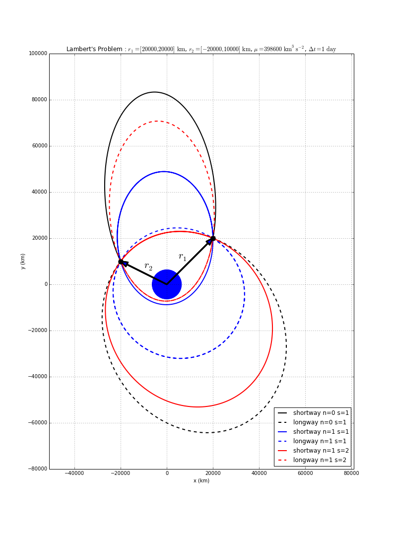
Lambert's problem is to solve for the orbit transfer that connects two position vectors in a given time of flight. It is one of the basic problems of orbital mechanics, and was solved by Swiss mathematician Johann Heinrich Lambert.

A standard Fortran 77 implementation of Lambert's problem was presented by Gooding [1]. A modern update to this implementation is included in the Fortran Astrodynamics Toolkit, which also includes a newer algorithm from Izzo [2].

There can be multiple solutions to Lambert's problem, which are classified by:

Direction of travel (i.e., a "short" way or "long" way transfer).
Number of complete revolutions (N=0,1,...). For longer flight times, solutions exist for larger values of N.
Solution number (S=1 or S=2). The multi-rev cases can have two solutions each.

In the example shown here, there are 6 possible solutions:

References

R.H, Gooding. "A procedure for the solution of Lambert's orbital boundary-value problem", Celestial Mechanics and Dynamical Astronomy, Vol. 48, No. 2, 1990.
D. Izzo, "Revisiting Lambert’s problem", Celestial Mechanics and Dynamical Astronomy, Oct. 2014.

posted at 03:14 · Programming · Fortran Lambert Orbital Mechanics

Fortran & C Interoperability

The ISO_C_BINDING intrinsic module and the BIND attribute introduced in Fortran 2003 are very handy for producing standard and portable Fortran code that interacts with C code. The example given here shows how to use the popen, fgets, and pclose routines from the C standard library to pipe the result of a shell command into a Fortran allocatable string.

module pipes_module

use,intrinsic :: iso_c_binding

implicit none

private

interface

    function popen(command, mode) bind(C,name='popen')
    import :: c_char, c_ptr
    character(kind=c_char),dimension(*) :: command
    character(kind=c_char),dimension(*) :: mode
    type(c_ptr) :: popen
    end function popen

    function fgets(s, siz, stream) bind(C,name='fgets')
    import :: c_char, c_ptr, c_int
    type (c_ptr) :: fgets
    character(kind=c_char),dimension(*) :: s
    integer(kind=c_int),value :: siz
    type(c_ptr),value :: stream
    end function fgets

    function pclose(stream) bind(C,name='pclose')
    import :: c_ptr, c_int
    integer(c_int) :: pclose
    type(c_ptr),value :: stream
    end function pclose

end interface

public :: c2f_string, get_command_as_string

contains

!**********************************************
! convert a C string to a Fortran string
!**********************************************
function c2f_string(c) result(f)

    implicit none

    character(len=*),intent(in) :: c
    character(len=:),allocatable :: f

    integer :: i

    i = index(c,c_null_char)

    if (i<=0) then
        f = c
    else if (i==1) then
        f = ''
    else if (i>1) then
        f = c(1:i-1)
    end if

end function c2f_string

!**********************************************
! return the result of the command as a string
!**********************************************
function get_command_as_string(command) result(str)

    implicit none

    character(len=*),intent(in) :: command
    character(len=:),allocatable :: str

    integer,parameter :: buffer_length = 1000

    type(c_ptr) :: h
    integer(c_int) :: istat
    character(kind=c_char,len=buffer_length) :: line

    str = ''
    h = c_null_ptr
    h = popen(command//c_null_char,'r'//c_null_char)

    if (c_associated(h)) then
        do while (c_associated(fgets(line,buffer_length,h)))
            str = str//c2f_string(line)
        end do
        istat = pclose(h)
    end if

end function get_command_as_string

end module pipes_module

A example use of this module is:

program test

use pipes_module

implicit none

character(len=:),allocatable :: res

res = get_command_as_string('uname')
write(*,'(A)') res

res = get_command_as_string('ls -l')
write(*,'(A)') res

end program test

References

C interop to popen, comp.lang.fortran, 12/2/2009.

posted at 19:03 · Programming · C Fortran Interoperability

Midpoint Circle Algorithm

circle

The Midpoint circle algorithm is a clever and efficient way of drawing a circle using only addition, subtraction, and bit shifts. It is based on the Bresenham line algorithm developed by Jack Bresenham in 1962 at IBM.

The algorithm was also independently discovered by Apple programmer Bill Atkinson in 1981 when developing QuickDraw for the original Macintosh.

A Fortran implementation is given below (which was used to draw the circle shown here, which has a radius of 7 pixels):

subroutine draw_circle(x0, y0, radius, color)

implicit none

integer,intent(in) :: x0, y0, radius, color

integer :: x,y,err

x = radius
y = 0
err = 1-x

do while (x >= y)

    call color_pixel( x + x0, y + y0, color)
    call color_pixel( y + x0, x + y0, color)
    call color_pixel( -x + x0, y + y0, color)
    call color_pixel( -y + x0, x + y0, color)
    call color_pixel( -x + x0, -y + y0, color)
    call color_pixel( -y + x0, -x + y0, color)
    call color_pixel( x + x0, -y + y0, color)
    call color_pixel( y + x0, -x + y0, color)

    y = y + 1

    if (err<0) then
        err = err + 2 * y + 1
    else
        x = x - 1
        err = err + 2 * (y - x + 1)
    end if

end do

end subroutine draw_circle

References

Jack E. Bresenham, "Algorithms for Computer Control of a Digital Plotter", IBM System Journal, 1965.

posted at 06:06 · Programming · Apple Fortran Graphics IBM

Python Fortran Rosetta Stone

Fortran90.org has a nice page showing side-by-side comparisons of the same code in both NumPy and Fortran. Aside from a few weird quirks (see the array slice examples), Python code should be easily understandable by a Fortran programmer.

posted at 13:55 · Programming · Fortran Python

Algorithms • Modern Fortran Programming • Orbital Mechanics

Feb 08, 2015

IAU Rotation Models

References

Jan 26, 2015

Nonsingular Geopotential Models

References

Jan 22, 2015

Julian Date

References

Dec 25, 2014

Merry Christmas

Dec 24, 2014

Fortran Build Tools

See also

Nov 22, 2014

Rocket Equation

References

Oct 30, 2014

Lambert's Problem

References

Oct 26, 2014

Fortran & C Interoperability

References

Oct 18, 2014

Midpoint Circle Algorithm

References

Sep 24, 2014

Python Fortran Rosetta Stone

References

- Stream Input/Output in Fortran [Fortran Wiki]
- Text file to allocatable string [Intel Fortran Forum] 03/03/2015
Feb 25, 2015
I just started a new modern Fortran software library called bspline-fortran, which is for multidimensional (multivariate) b-spline interpolation of data defined on a regular grid. It is available on GitHub, and released under a permissive BSD-style license.
It seems impossible to find code for higher than 3D spline interpolation on the internet. Einspline only has 1D-3D, as do the NIST Core Math Library DBSPLIN and DTENSBS routines. Python's SciPy stops at 2D (Bivariate splines). At first glance, the SciPy routine map_coordinates seems to do what I want, but not really since there doesn't seem to be any way to specify the abscissa vectors (x, y, z, etc.). Note: maybe there is a way, but looking at the less-than-great documentation, the minimally-commented C code, and then reading several confusing Stack Overflow posts didn't help me much. Apparently, I'm not the only one confused by this routine.
After much searching, I finally just took the 2D and 3D NIST routines (written in 1982), refactored them significantly so I could better understand what they were doing, and then extended the algorithm into higher dimensions (which is actually quite easy to do for b-splines). The original FORTRAN 77 code was somewhat hard to follow, since it was stuffing matrices into a giant WORK vector, which required a lot of obscure bookkeeping of indices. For example, I replaced this bit of code:
IZM1 = IZ - 1
KCOLY = LEFTY - KY + 1
DO 60 K=1,KZ
I = (K-1)*KY + 1
J = IZM1 + K
WORK(J) = DBVALU(TY(KCOLY),WORK(I),KY,KY,IDY,YVAL,INBV1,WORK(IW))
60  CONTINUE
with this:
kcoly = lefty - ky + 1
do k=1,kz
temp2(k) = dbvalu(ty(kcoly:),temp1(:,k),ky,ky,idy,yval,inbv1,work)
end do
which makes it a lot easier to deal with and add the extra dimensions as necessary.
The new library contains routines for 2D, 3D, 4D, 5D, and 6D interpolation. It seems like someone else may find them useful, I don't know why they don't seem to be available anywhere else. Eventually, I'll add object-oriented wrappers for the core routines, to make them easier to use.
Feb 16, 2015
I just came across this article from 2005 written by Jef Raskin (probably most famous for having initiated the Macintosh project at Apple) on source code documentation [1]. I agree with much of what he recommends. I have never believed that code can be "self-documenting" without comments, and generally will start writing the comments before I start the actual code. I also like some aspects of Knuth's "literate programming" concept [2].
I do find automatic documentation generators useful, however. There aren't a lot of solutions for modern Fortran projects though. I've not tried to use Doxygen, but am told that support for modern Fortran features is somewhat lacking [3]. ROBODoc is pretty good, although it does not perform any code analysis, and only extracts specific comment blocks that you indicate in the source. A brand new tool called ford is very promising, since it was created with modern Fortran in mind.
I also have an idea that the best code (including comments) should be understandable to a reasonably intelligent person who is not familiar with the programming language. Some languages (Fortran, Python) make this easier than others (C++, Haskell). There is a good article here, discussing the "beauty" of some C++ code (although I disagree with his views on comments). I was struck by the discussion on how to write functions so that more information is provided to the reader of the code [4]. The example given is this:
int idSurface::Split( const idPlane &plane, const float epsilon,
idSurface **front, idSurface **back,
int *frontOnPlaneEdges, int *backOnPlaneEdges ) const;
Of course, if you are not familiar with the C++ *, **, and & characters and the const declaration, there is no information you can derive from this. It is complete gibberish. Modern Fortran, on the other hand, provides for the declaration of an intent attribute to function and subroutine arguments. The equivalent Fortran version would look something like this:
integer function split(me,plane,eps,front,back,&
frontOnPlaneEdges,backOnPlaneEdges)
class(idSurface),intent(in) :: me
type(idPlane), intent(in) :: plane
real, intent(in) :: eps
type(idSurface), intent(out) :: front
type(idSurface), intent(out) :: back
integer, intent(out) :: frontOnPlaneEdges
integer, intent(out) :: backOnPlaneEdges
Here, it should be more obvious what is happening (for example, that plane is an input and front is an output). The use of words rather than symbols definitely improves readability for the non-expert (although if taken to the extreme, you would end up with COBOL).
- J. Raskin, "Comments are More Important than Code", Queue, Volume 3 Issue 2, March 2005, Pages 64-65.
- D. E. Knuth, "Literate Programming", The Computer Journal (1984) 27 (2): 97-111.
- F03/08 supporting Documentation tools, comp.lang.fortran.
- S. McGrath, "The Exceptional Beauty of Doom 3's Source Code", kotaku.com, Jan. 14, 2013.