Degenerate Conic

Fortran and Pyplot

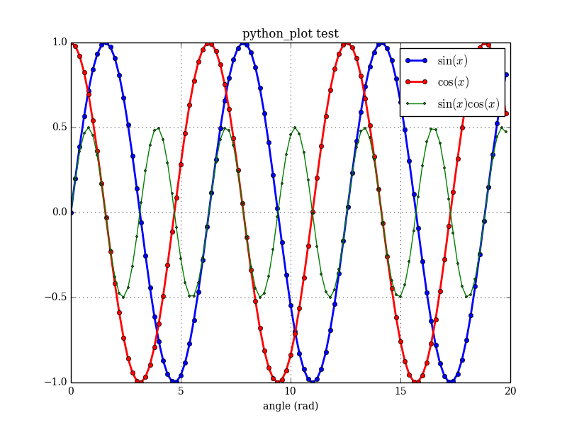
Python's matplotlib.pyplot is a very nice collection of functions that provide an easy Matlab-like interface for data plotting. It can be used to generate quite professional looking plots. There is a lot of information on the internet about calling Fortran from Python, but what if all you want to do is generate some plots from your (modern) Fortran program? With this in mind, I've created a very simple Fortran wrapper for Pyplot, allowing you to make pretty good plots by writing only Fortran code. Consider the following example:

program test

use,intrinsic :: iso_fortran_env, only: wp => real64
use pyplot_module

implicit none

real(wp),dimension(100) :: x,sx,cx,tx
type(pyplot) :: plt
integer :: i

!generate some data:
x = [(real(i,wp), i=0,size(x)-1)]/5.0_wp
sx = sin(x)
cx = cos(x)
tx = sx * cx

!plot it:
call plt%initialize(grid=.true.,xlabel='angle (rad)',&
                    title='python_plot test',legend=.true.)
call plt%add_plot(x,sx,label='\$\sin (x)\$',&
                  linestyle='b-o',markersize=5,linewidth=2)
call plt%add_plot(x,cx,label='\$\cos (x)\$',&
                  linestyle='r-o',markersize=5,linewidth=2)
call plt%add_plot(x,tx,label='\$\sin (x) \cos (x)\$',&
                  linestyle='g-o',markersize=2,linewidth=1)
call plt%savefig('test.png')

end program test

The main user interface is the pyplot class, which has methods such as initialize, add_plot, and savefig. This example produces the following plot:

All the module does is generate a Python script, and then runs it and saves the result. The Python call is completely transparent to the Fortran user.

I posted the project to GitHub (pyplot-fortran). Maybe someone else will find it useful, or help to expand it.

See also

1. matplotlib
2. F2PY Users Guide and Reference Manual --Fortran to Python interface generator

Lagrange Interpolating Polynomials

A simple Fortran implementation of interpolation by Lagrange polynomials is given below. Though named after Joseph-Louis Lagrange, the formula was first discovered by English mathematician Edward Waring.

subroutine lagrange_interpolation(xx,yy,x,y)
!
! Interpolate xx=[x1,x2,...xn]
! yy=[f(x1),f(x2),...,f(xn)]
! Using Lagrange polynomial P(x)
! Returns y = P(x)
!
use,intrinsic :: iso_fortran_env, wp => real64

implicit none

real(wp),dimension(:),intent(in) :: xx
real(wp),dimension(:),intent(in) :: yy
real(wp),intent(in) :: x
real(wp),intent(out) :: y

!local variables:
integer :: j,k,n,m
real(wp) :: p

!check number of points:
n = size(xx)
m = size(yy)
if (n/=m) error stop &
    'Error: vectors must be the same size.'

!sum each of the Pj(x) terms:
y = 0.0_wp
do j=1,n
    !compute Pj(x):
    p = yy(j)
    do k=1,n
        if (k/=j) p = p * (x-xx(k)) / (xx(j)-xx(k))
    end do
    y = y + p
end do

end subroutine lagrange_interpolation

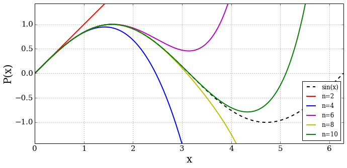
Examples of interpolating polynomials for the \(\sin(x)\) function are shown here for different numbers of points \(x=[0.0, 0.01]\), \(x=[0.0, 0.01, 0.02]\), etc.

References

• Lagrange Interpolating Polynomial [Wolfram Mathworld]
• E. Waring, "Problems Concerning Interpolations", Philosophical Transactions of the Royal Society of London, Vol. 69 (1779), p. 59-67.

Too Much Confusion

There is a lot of confusion and misinformation about the Fortran programming language on the internet, and a general ignorance about it among programmers. Most younger programmers who use languages invented five minutes ago probably have never seen it, and may only be dimly aware of it as some obsolete language that nobody uses anymore.

You may be surprised to learn that Fortran is a modern, object-oriented, general-purpose programming language. Fortran is not a programming language created by computer scientists to write operating systems, nor does it include every single programming concept anyone's ever heard of. It is a language designed for computational efficiency and efficient array manipulation, and has a clear uncluttered syntax that can be read and understood by non-experts with only a little effort and training. It is particularly suited for numerical and scientific programming by non-expert programmers such as engineers and scientists. Learning all of Fortran is considerably easier than learning all of C++ (as an example). Sure, you can't do template metaprogramming, but few engineer/scientist types would ever want to do that anyway (besides, it's bad for you and could make you go blind).

By "Fortran", I mean modern Fortran (i.e., Fortran 2003 and 2008, which is the latest standard). Yes, the roots of Fortran go way back to the 1950s. Sure, early Fortran programs were written on punched cards. So what? Latin was once scratched into wax tablets, but that isn't really relevant to modern Italian and French speakers. In fact, the Fortran language has evolved considerably since it was first standardized in 1966. It generally has followed a cycle where a major update is followed by a minor update (1977=minor, 1990=major, 1995=minor, 2003=major, 2008=minor). It has been said that the 2003 update was as big an update to Fortran 95 as C++ was to C! Ten years later, the GNU Fortran compiler is still not fully F2003 compliment (the Intel compiler only recently became so).

People who attempt to enter the world of Fortran programming are easily corrupted and discouraged by misinformation. Even a lot of old-school Fortran users are unaware of the later standards. This is too bad, because modern Fortran is actually quite a respectable programming language for a lot of technical applications. This article is a pretty good overview of Fortran for C/C++ programmers. However, it is outdated, since it is confined to Fortran 95. Most of the limitations it mentions (no procedure pointers, clunky character strings, lack of an intent attribute for pointer dummy arguments, the nonstandardness of the ; character) have been rectified in subsequent standards.

The fact is the internet is not really the best source of information for modern Fortran. One day, maybe, there will be vibrant community of Fortran users on the internet, extensive online documentation, open source projects, and all your questions will simply be a web search away (cf., Python). But for now, you'll probably have to buy some books. If a book has the numbers 77, 90, or 95 in the title, don't open it, it will only confuse you. This is not to say that there aren't friendly Fortran folk on the internet who will also help you out. Two of the best places to go with questions are the Intel Fortran forum and the comp.lang.fortran newsgroup (yes, apparently, Usenet still exists).

References

• N. Maclaren, Why (and Why Not) to Use Fortran: Instead of C++, Matlab, Python etc., University of Cambridge Computing Service, June 2012.
• L. Phillips, Scientific computing’s future: Can any coding language top a 1950s behemoth?, May 7, 2014 [arstechnica.com]
• Fortran Wiki -- an open venue for discussing all aspects of the Fortran programming language and scientific computing.
• A. Koenig, C Traps and Pitfalls, AT&T Bell Laboratories.
• Why C and C++ are Awful Programming Languages

json-fortran 4.0.0

I just tagged the 4.0.0 release of json-fortran. This is the first release with Unicode support (thanks to Izaak Beekman). Who says there are no good open source Fortran projects on the internet?

The Unicode build of the library is optional (and only enabled using the preprocessor directive USE_UCS4). Currently, this only works with Gfortran. It doesn't yet work with the Intel Fortran Compiler, which is lagging behind on Unicode support. The Fortran standard supports Unicode via the selected_char_kind function, which can be used to specify the character set used for a character string, like so:

integer,parameter :: u = selected_char_kind('ISO_10646')
character(kind=u,len=11) :: string = u_'Hello World'

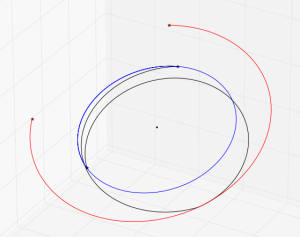
Earth-Mars Free Return

Let's try using the Fortran Astrodynamics Toolkit and Pikaia to solve a real-world orbital mechanics problem. In this case, computing the optimal Earth-Mars free return trajectory in the year 2018. This is a trajectory that departs Earth, and then with no subsequent maneuvers, flies by Mars and returns to Earth. The building blocks we need to do this are:

1. An ephemeris of the Earth and Mars [DE405]
2. A Lambert solver [1]
3. Some equations for hyperbolic orbits [given below]
4. An optimizer [Pikaia]

The \(\mathbf{v}_{\infty}\) vector of a hyperbolic planetary flyby (using patched conic assumptions) is simply the difference between the spacecraft's heliocentric velocity and the planet's velocity:

• \(\mathbf{v}_{\infty} = \mathbf{v}_{heliocentric} - \mathbf{v}_{planet}\)

The hyperbolic turning angle \(\Delta\) is the angle between \(\mathbf{v}_{\infty}^{-}\) (the \(\mathbf{v}_{\infty}\) before the flyby) and the \(\mathbf{v}_{\infty}^{+}\) (the \(\mathbf{v}_{\infty}\) vector after the flyby). The turning angle can be used to compute the flyby periapsis radius \(r_p\) using the equations:

• \(e = \frac{1}{\sin(\Delta/2)}\)
• \(r_p = \frac{\mu}{v_{\infty}^2}(e-1)\)

So, from the Lambert solver, we can obtain Earth to Mars, and Mars to Earth trajectories (and the heliocentric velocities at each end). These are used to compute the \(\mathbf{v}_{\infty}\) vectors at: Earth departure, Mars flyby (both incoming and outgoing vectors), and Earth return.

There are three optimization variables:

• The epoch of Earth departure [modified Julian date]
• The outbound flight time from Earth to Mars [days]
• The return flyby time from Mars to Earth [days]

There are also two constraints on the heliocentric velocity vectors before and after the flyby at Mars:

• The Mars flyby must be unpowered (i.e., no propulsive maneuver is performed). This means that the magnitude of the incoming (\(\mathbf{v}_{\infty}^-\)) and outgoing (\(\mathbf{v}_{\infty}^+\)) vectors must be equal.
• The periapsis flyby radius (\(r_p\)) must be greater than some minimum value (say, 160 km above the Martian surface).

For the objective function (the quantity that is being minimized), we will use the sum of the Earth departure and return \(\mathbf{v}_{\infty}\) vector magnitudes. To solve this problem using Pikaia, we need to create a fitness function, which is given below:

subroutine obj_func(me,x,f)

!Pikaia fitness function for an Earth-Mars free return

use fortran_astrodynamics_toolkit

implicit none

class(pikaia_class),intent(inout) :: me !pikaia class
real(wp),dimension(:),intent(in) :: x !optimization variable vector
real(wp),intent(out) :: f !fitness value

real(wp),dimension(6) :: rv_earth_0, rv_mars, rv_earth_f
real(wp),dimension(3) :: v1,v2,v3,v4,vinf_0,vinf_f,vinfm,vinfp
real(wp) :: jd_earth_0,jd_mars,jd_earth_f,&
dt_earth_out,dt_earth_return,&
rp_penalty,vinf_penalty,e,delta,rp,vinfmag

real(wp),parameter :: mu_sun = 132712440018.0_wp !sun grav param [km3/s2]
real(wp),parameter :: mu_mars = 42828.0_wp !mars grav param [km3/s2]
real(wp),parameter :: rp_mars_min = 3390.0_wp+160.0_wp !min flyby radius at mars [km]
real(wp),parameter :: vinf_weight = 1000.0_wp !weights for the
real(wp),parameter :: rp_weight = 10.0_wp ! penalty functions

!get times:
jd_earth_0 = mjd_to_jd(x(1)) !julian date of earth departure
dt_earth_out = x(2) !outbound flyby time [days]
dt_earth_return = x(3) !return flyby time [days]
jd_mars = jd_earth_0 + dt_earth_out !julian date of mars flyby
jd_earth_f = jd_mars + dt_earth_return !julian date of earth arrival

!get earth/mars locations (wrt Sun):
call get_state(jd_earth_0,3,11,rv_earth_0) !earth at departure
call get_state(jd_mars, 4,11,rv_mars) !mars at flyby
call get_state(jd_earth_f,3,11,rv_earth_f) !earth at arrival

!compute lambert maneuvers:
call lambert(rv_earth_0,rv_mars, dt_earth_out*day2sec, mu_sun,v1,v2) !outbound
call lambert(rv_mars, rv_earth_f,dt_earth_return*day2sec,mu_sun,v3,v4) !return

!compute v-inf vectors:
vinf_0 = v1 - rv_earth_0(4:6) !earth departure
vinfm = v2 - rv_mars(4:6) !mars flyby (incoming)
vinfp = v3 - rv_mars(4:6) !mars flyby (outgoing)
vinf_f = v4 - rv_earth_f(4:6) !earth return

!the turning angle is the angle between vinf- and vinf+
delta = angle_between_vectors(vinfm,vinfp) !turning angle [rad]
vinfmag = norm2(vinfm) !vinf vector mag (incoming) [km/s]
e = one/sin(delta/two) !eccentricity
rp = mu_mars/(vinfmag*vinfmag)*(e-one) !periapsis radius [km]

!the constraints are added to the fitness function as penalties:
if (rp>=rp_mars_min) then
    rp_penalty = zero !not active
else
    rp_penalty = rp_mars_min - rp
end if
vinf_penalty = abs(norm2(vinfm) - norm2(vinfp))

!fitness function (to maximize):
f = - ( norm2(vinf_0) + &
    norm2(vinf_f) + &
    vinf_weight*vinf_penalty + &
    rp_weight*rp_penalty )

end subroutine obj_func

The lambert routine called here is simply a wrapper to solve_lambert_gooding that computes both the "short way" and "long way" transfers, and returns the one with the lowest total \(\Delta v\). The two constraints are added to the objective function as penalties (to be driven to zero). Pikaia is then initialized and called by:

program flyby

use pikaia_module
use fortran_astrodynamics_toolkit

implicit none

integer,parameter :: n = 3

type(pikaia_class) :: p
real(wp),dimension(n) :: x,xl,xu
integer :: status,iseed
real(wp) :: f

!set random number seed:
iseed = 371

!bounds:
xl = [jd_to_mjd(julian_date(2018,1,1,0,0,0)), 100.0_wp,100.0_wp]
xu = [jd_to_mjd(julian_date(2018,12,31,0,0,0)),400.0_wp,400.0_wp]

call p%init(n,xl,xu,obj_func,status,&
            ngen = 1000, &
            np = 200, &
            nd = 9, &
            ivrb = 0, &
            convergence_tol = 1.0e-6_wp, &
            convergence_window = 200, &
            initial_guess_frac = 0.0_wp, &
            iseed = iseed )

call p%solve(x,f,status)

end program flyby

The three optimization variables are bounded: the Earth departure epoch must occur sometime in 2018, and the outbound and return flight times must each be between 100 and 400 days.

Running this program, we can get different solutions (depending on the value set for the random seed, and also the Pikaia settings). The best one I've managed to get with minimal tweaking is this:

• Earth departure epoch: MJD 58120 (Jan 2, 2018)
• Outbound flight time: 229 days
• Return flight time: 271 days

Which is similar to the solution shown in [2].

References

1. R.H. Gooding, "A procedure for the solution of Lambert's orbital boundary-value problem", Celestial Mechanics and Dynamical Astronomy, Vol. 48, No. 2, 1990.
2. Dennis Tito's 2021 Human Mars Flyby Mission Explained. SPACE.com, February 27, 2014.
3. J.E. Prussing, B.A. Conway, "Orbital Mechanics", Oxford University Press, 1993.

Pikaia

I've started a new project on Github for a new modern object-oriented version of the Pikaia genetic algorithm code. This is a refactoring and upgrade of the Pikaia code from the High Altitude Observatory. The original code is public domain and was written by Paul Charbonneau & Barry Knapp (version 1.2 was released in 2003). The new code differs from the old code in the following respects:

• The original fixed-form source (FORTRAN 77) was converted to free-form source.
• The code is now object-oriented Fortran 2003/2008. All user interaction is now through a class, which is the only public entity in the module.
• All real variables are now 8 bytes (a.k.a. "double precision"). The precision can also be changed by the user by modifying the wp parameter.
• The random number generator was replaced with calls to the intrinsic Fortran random_number function.
• There are various new options (e.g., a convergence window with a tolerance can be specified as a stopping condition, and the user can specify a subroutine for reporting the best solution at each generation).
• Mapping the variables to be between 0 and 1 now occurs internally, rather than requiring the user to do it.
• Can now include an initial guess in the initial population.

This is another example of how older Fortran codes can be refactored to bring them up to date with modern computing concepts without doing that much work. In my opinion, the object-oriented Fortran 2003 interface is a lot better than the old FORTRAN 77 version. For one, it's easier to follow. Also, data can now easily be passed into the user fitness function by extending the pikaia class and putting the data there. No common blocks necessary!

References

1. Original Pikaia code and documentation [High Altitude Observatory]

Fortran Stream I/O

Fortran 2003 introduced many new features to the language that make things a lot easier than they were in the bad old days. Deferred-length character strings and stream I/O are two examples. Deferred-length strings were a huge addition, since they allow the length of character variables to be resized on-the-fly, something never before possible in Fortran. (Note: if you happen to come across a Fortran 90 monstrosity called ISO_VARYING_STRING, avoid it like the plague. That is not what I'm talking about.) Stream I/O is also quite handy, allowing you to access files as a stream of bytes or characters. The following example uses both features to create a subroutine that reads in the contents of a text file into an allocatable string. Note that it uses the size argument of the intrinsic inquire function to get the file size before allocating the string.

subroutine read_file(filename,str)  
!  
! Reads the contents of the file into the allocatable string str.  
! If there are any problems, str will be returned unallocated.  
!  
implicit none

character(len=*),intent(in) :: filename  
character(len=:),allocatable,intent(out) :: str

integer :: iunit,istat,filesize

open(newunit=iunit,file=filename,status='OLD',&  
form='UNFORMATTED',access='STREAM',iostat=istat)

if (istat==0) then  
    inquire(file=filename, size=filesize)  
    if (filesize>0) then  
        allocate( character(len=filesize) :: str )  
        read(iunit,pos=1,iostat=istat) str  
        if (istat/=0) deallocate(str)  
        close(iunit, iostat=istat)  
    end if  
end if

end subroutine read_file  

References

1. Stream Input/Output in Fortran [Fortran Wiki]
2. Text file to allocatable string [Intel Fortran Forum] 03/03/2015

Multidimensional B-Spline Interpolation

I just started a new modern Fortran software library called bspline-fortran, which is for multidimensional (multivariate) b-spline interpolation of data defined on a regular grid. It is available on GitHub, and released under a permissive BSD-style license.

It seems impossible to find code for higher than 3D spline interpolation on the internet. Einspline only has 1D-3D, as do the NIST Core Math Library DBSPLIN and DTENSBS routines. Python's SciPy stops at 2D (Bivariate splines). At first glance, the SciPy routine map_coordinates seems to do what I want, but not really since there doesn't seem to be any way to specify the abscissa vectors (x, y, z, etc.). Note: maybe there is a way, but looking at the less-than-great documentation, the minimally-commented C code, and then reading several confusing Stack Overflow posts didn't help me much. Apparently, I'm not the only one confused by this routine.

After much searching, I finally just took the 2D and 3D NIST routines (written in 1982), refactored them significantly so I could better understand what they were doing, and then extended the algorithm into higher dimensions (which is actually quite easy to do for b-splines). The original FORTRAN 77 code was somewhat hard to follow, since it was stuffing matrices into a giant WORK vector, which required a lot of obscure bookkeeping of indices. For example, I replaced this bit of code:

    IZM1 = IZ - 1  
    KCOLY = LEFTY - KY + 1  
    DO 60 K=1,KZ  
      I = (K-1)*KY + 1  
      J = IZM1 + K  
      WORK(J) = DBVALU(TY(KCOLY),WORK(I),KY,KY,IDY,YVAL,INBV1,WORK(IW))  
60  CONTINUE  

with this:

kcoly = lefty - ky + 1  
do k=1,kz  
    temp2(k) = dbvalu(ty(kcoly:),temp1(:,k),ky,ky,idy,yval,inbv1,work)  
end do  

which makes it a lot easier to deal with and add the extra dimensions as necessary.

The new library contains routines for 2D, 3D, 4D, 5D, and 6D interpolation. It seems like someone else may find them useful, I don't know why they don't seem to be available anywhere else. Eventually, I'll add object-oriented wrappers for the core routines, to make them easier to use.

Comments

I just came across this article from 2005 written by Jef Raskin (probably most famous for having initiated the Macintosh project at Apple) on source code documentation [1]. I agree with much of what he recommends. I have never believed that code can be "self-documenting" without comments, and generally will start writing the comments before I start the actual code. I also like some aspects of Knuth's "literate programming" concept [2].

I do find automatic documentation generators useful, however. There aren't a lot of solutions for modern Fortran projects though. I've not tried to use Doxygen, but am told that support for modern Fortran features is somewhat lacking [3]. ROBODoc is pretty good, although it does not perform any code analysis, and only extracts specific comment blocks that you indicate in the source. A brand new tool called ford is very promising, since it was created with modern Fortran in mind.

I also have an idea that the best code (including comments) should be understandable to a reasonably intelligent person who is not familiar with the programming language. Some languages (Fortran, Python) make this easier than others (C++, Haskell). There is a good article here, discussing the "beauty" of some C++ code (although I disagree with his views on comments). I was struck by the discussion on how to write functions so that more information is provided to the reader of the code [4]. The example given is this:

int idSurface::Split( const idPlane &plane, const float epsilon,  
                      idSurface **front, idSurface **back,  
                      int *frontOnPlaneEdges, int *backOnPlaneEdges ) const;  

Of course, if you are not familiar with the C++ *, **, and & characters and the const declaration, there is no information you can derive from this. It is complete gibberish. Modern Fortran, on the other hand, provides for the declaration of an intent attribute to function and subroutine arguments. The equivalent Fortran version would look something like this:

integer function split(me,plane,eps,front,back,&  
                       frontOnPlaneEdges,backOnPlaneEdges)

class(idSurface),intent(in) :: me  
type(idPlane), intent(in) :: plane  
real, intent(in) :: eps  
type(idSurface), intent(out) :: front  
type(idSurface), intent(out) :: back  
integer, intent(out) :: frontOnPlaneEdges  
integer, intent(out) :: backOnPlaneEdges  

Here, it should be more obvious what is happening (for example, that plane is an input and front is an output). The use of words rather than symbols definitely improves readability for the non-expert (although if taken to the extreme, you would end up with COBOL).

References

1. J. Raskin, "Comments are More Important than Code", Queue, Volume 3 Issue 2, March 2005, Pages 64-65.
2. D. E. Knuth, "Literate Programming", The Computer Journal (1984) 27 (2): 97-111.
3. F03/08 supporting Documentation tools, comp.lang.fortran.
4. S. McGrath, "The Exceptional Beauty of Doom 3's Source Code", kotaku.com, Jan. 14, 2013.

IAU Rotation Models

The IAU Working Group on Cartographic Coordinates and Rotational Elements (WGCCRE) is the keeper of official models that describe the cartographic coordinates and rotational elements of planetary bodies (such as the Earth, satellites, minor planets, and comets). Periodically, they release a report containing the coefficients to compute body orientations, based on the latest data available. These coefficients allow one to compute the rotation matrix from the ICRF frame to a body-fixed frame (for example, IAU Earth) by giving the direction of the pole vector and the prime meridian location as functions of time. An example Fortran module illustrating this for the IAU Earth frame is given below. The coefficients are taken from the 2009 IAU report [Reference 1]. Note that the IAU models are also available in SPICE (as "IAU_EARTH", "IAU_MOON", etc.). For Earth, the IAU model is not suitable for use in applications that require the highest possible accuracy (for that a more complex model would be necessary), but is quite acceptable for many applications.

module iau_orientation_module

use, intrinsic :: iso_fortran_env, only: wp => real64

implicit none

private

!constants:
real(wp),parameter :: zero = 0.0_wp
real(wp),parameter :: one = 1.0_wp
real(wp),parameter :: pi = acos(-one)
real(wp),parameter :: pi2 = pi/2.0_wp
real(wp),parameter :: deg2rad = pi/180.0_wp
real(wp),parameter :: sec2day = one/86400.0_wp
real(wp),parameter :: sec2century = one/3155760000.0_wp

public :: icrf_to_iau_earth

contains

!Rotation matrix from ICRF to IAU_EARTH
pure function icrf_to_iau_earth(et) result(rotmat)

implicit none

real(wp),intent(in) :: et !ephemeris time [sec from J2000]
real(wp),dimension(3,3) :: rotmat !rotation matrix

real(wp) :: w,dec,ra,d,t
real(wp),dimension(3,3) :: tmp

d = et * sec2day !days from J2000
t = et * sec2century !Julian centuries from J2000

ra = ( - 0.641_wp * t ) * deg2rad
dec = ( 90.0_wp - 0.557_wp * t ) * deg2rad
w = ( 190.147_wp + 360.9856235_wp * d ) * deg2rad

!it is a 3-1-3 rotation:
tmp = matmul( rotmat_x(pi2-dec), rotmat_z(pi2+ra) )
rotmat = matmul( rotmat_z(w), tmp )

end function icrf_to_iau_earth

!The 3x3 rotation matrix for a rotation about the x-axis.
pure function rotmat_x(angle) result(rotmat)

implicit none

real(wp),dimension(3,3) :: rotmat !rotation matrix
real(wp),intent(in) :: angle !angle [rad]

real(wp) :: c,s

c = cos(angle)
s = sin(angle)

rotmat = reshape([one, zero, zero, &
                  zero, c, -s, &
                  zero, s, c],[3,3])

end function rotmat_x

!The 3x3 rotation matrix for a rotation about the z-axis.
pure function rotmat_z(angle) result(rotmat)

implicit none

real(wp),dimension(3,3) :: rotmat !rotation matrix
real(wp),intent(in) :: angle !angle [rad]

real(wp) :: c,s

c = cos(angle)
s = sin(angle)

rotmat = reshape([ c, -s, zero, &
                   s, c, zero, &
                   zero, zero, one ],[3,3])

end function rotmat_z

end module iau_orientation_module

References

1. B. A. Archinal, et al., "Report of the IAU Working Group on Cartographic Coordinates and Rotational Elements: 2009", Celest Mech Dyn Astr (2011) 109:101-135.
2. J. Williams, Fortran Astrodynamics Toolkit - iau_orientation_module [GitHub]