Apr 28, 2016

Gfortran 6.1 (part of GCC) has been released. The release notes don't say much with respect to Fortran:
- The
MATMUL intrinsic is now inlined for straightforward cases if front-end optimization is active. The maximum size for inlining can be set to n with the -finline-matmul-limit=n option and turned off with -finline-matmul-llimit=0.
- The
-Wconversion-extra option will warn about REAL constants which have excess precision for their kind.
- The
-Winteger-division option has been added, which warns about divisions of integer constants which are truncated. This option is included in -Wall by default.
But, apparently, this version includes some nice updates, including support for Fortran 2008 submodules, Fortran 2015 Coarray events, as well as bug fixes for deferred-length character variables.
See also
Apr 24, 2016

Here's another example using the C interoperability features of modern Fortran. First introduced in Fortran 2003, this allows for easily calling C routines from Fortran (and vice versa) in a standard and portable way. Further interoperability features will also be added in the next edition of the standard.
For a Fortran user, strings in C are pretty awful (like most things in C). This example shows how to call a C function that returns a string (in this case, the dlerror function).
module get_error_module

use, intrinsic :: iso_c_binding

implicit none

private

public :: get_error

interface
    !interfaces to C functions
    function dlerror() result(error) &
    bind(C, name='dlerror')
    import
    type(c_ptr) :: error
    end function dlerror

    function strlen(str) result(isize) &
    bind(C, name='strlen')
    import
    type(c_ptr),value :: str
    integer(c_int) :: isize
    end function strlen
end interface

contains

function get_error() result(error_message)
!! wrapper to C function char *dlerror(void);

character(len=:),allocatable :: error_message

type(c_ptr) :: cstr
integer(c_int) :: n

cstr = dlerror() ! pointer to C string

if (c_associated(cstr)) then

    n = strlen(cstr) ! get string length

    block
        !convert the C string to a Fortran string
        character(kind=c_char,len=n+1),pointer :: s
        call c_f_pointer(cptr=cstr,fptr=s)
        error_message = s(1:n)
        nullify(s)
    end block

else
    error_message = ''
end if

end function get_error

end module get_error_module
First we define the bindings to two C routines so that we can call them from Fortran. This is done using the INTERFACE block. The main one is the dlerror function itself, and we will also use the C strlen function for getting the length of a C string. The bind(C) attribute indicates that they are C functions. The get_error function first calls dlerror, which returns a variable of type(c_ptr), which is a C pointer. We use c_f_pointer to cast the C pointer into a Fortran character string (a CHARACTER pointer variable with the same length). Note that, after we know the string length, the block construct allows us to declare a new variable s of the length we need (this is a Fortran 2008 feature). Then we can use it like any other Fortran string (in this case, we assign it to error_message, the deferred-length string returned by the function).
Of course, Fortran strings are way easier to deal with, especially deferred-length (allocatable) strings, and don't require screwing around with pointers or '\0' characters. A few examples are given below:
subroutine string_examples()

implicit none

!declare some strings:
character(len=:),allocatable :: s1,s2

!string assignment:
s1 = 'hello world' !set the string value
s2 = s1 !set one string equal to another

!string slice:
s1 = s1(1:5) !now, s1 is 'hello'

!string concatenation:
s2 = s1//' '//s1 ! now, s2 is 'hello hello'

!string length:
write(*,*) len(s2) ! print length of s2 (which is now 11)

!and there are no memory leaks,
!since the allocatables are automatically
!deallocated when they go out of scope.

end subroutine string_examples
See also
Apr 09, 2016
Built-in high-level support for arrays (vectors and matrices) using a very clean syntax is one of the areas where Fortran really shines as a programming language for engineering and scientific simulations. As an example, consider matrix multiplication. Say we have an M x K matrix A, a K x N matrix B, and we want to multiply them to get the M x N matrix AB. Here's the code to do this in Fortran:
Now, here's how to do the same thing in C or C++ (without resorting to library calls) [1]:
for (int i = 0; i < M; i++) {
    for (int j = 0; j < N; j++) {
        AB[i][j]=0;
        for (int k = 0; k < K; k++) {
            AB[i][j] += A[i][k] * B[k][j];
        }
    }
}
MATMUL is, of course, Fortran's built-in matrix multiplication function. It was added to the language as part of the Fortran 90/95 standards which dramatically upgraded the language's array-handling facilities. Later standards also added additional array features, and Fortran currently contains a wide range of intrinsic array functions:
| Routine |
Description |
| ALL |
True if all values are true |
| ALLOCATED |
Array allocation status |
| ANY |
True if any value is true |
| COUNT |
Number of true elements in an array |
| CSHIFT |
Circular shift |
| DOT_PRODUCT |
Dot product of two rank-one arrays |
| EOSHIFT |
End-off shift |
| FINDLOC |
Location of a specified value |
| IPARITY |
Exclusive or of array elements |
| IS_CONTIGUOUS |
Test contiguity of an array |
| LBOUND |
Lower dimension bounds of an array |
| MATMUL |
Matrix multiplication |
| MAXLOC |
Location of a maximum value in an array |
| MAXVAL |
Maximum value in an array |
| MERGE |
Merge under mask |
| MINLOC |
Location of a minimum value in an array |
| MINVAL |
Minimum value in an array |
| NORM2 |
L2 norm of an array |
| PACK |
Pack an array into an array of rank one under a mask |
| PARITY |
True if number of elements in odd |
| PRODUCT |
Product of array elements |
| RESHAPE |
Reshape an array |
| SHAPE |
Shape of an array or scalar |
| SIZE |
Total number of elements in an array |
| SPREAD |
Replicates array by adding a dimension |
| SUM |
Sum of array elements |
| TRANSPOSE |
Transpose of an array of rank two |
| UBOUND |
Upper dimension bounds of an array |
| UNPACK |
Unpack an array of rank one into an array under a mask |
As an example, here is how to sum all the positive values in a matrix:
In addition to the array-handling functions, we can also use various other language features to make it easier to work with arrays. For example, say we wanted to convert all the negative elements of a matrix to zero:
Or, say we want to compute the dot product of the 1st and 3rd columns of a matrix:
d = dot_product(A(:,1),A(:,3))
Or, replace every element of a matrix with its sin():
That last one is an example of an intrinsic ELEMENTAL function, which is one that can operate on scalars or arrays of any rank. The assignment is done for each element of the array (and can potentially be vectored by the compiler). We can create our own ELEMENTAL functions like so:
elemental function cubic(a,b,c) result(d)
real(wp),intent(in) :: a,b,c
real(wp) :: d
d = a + b**2 + c**3
end function cubic
Note that the inputs and output of this function are scalars. However, since it is ELEMENTAL, it can also be used for arrays like so:
real(wp) :: aa,bb,cc,dd
real(wp),dimension(10,10,10) :: a,b,c,d
!...
dd = cubic(aa,bb,cc) ! works on these
d = cubic(a,b,c) ! also works on these
The array-handling features of Fortran make scientific and engineering programming simpler and less error prone, since the code can be closer to the mathematical expressions, as well as making vectorization by the compiler easier [2]. Here is an example from the Fortran Astrodynamics Toolkit, a vector projection function:
pure function vector_projection(a,b) result(c)

implicit none

real(wp),dimension(:),intent(in) :: a
!! the original vector
real(wp),dimension(size(a)),intent(in) :: b
!! the vector to project on to
real(wp),dimension(size(a)) :: c
!! the projection of a onto b

if (all(a==0.0_wp)) then
    c = 0.0_wp
else
    c = a * dot_product(a,b) / dot_product(a,a)
end if

end function vector_projection
Line 15 is the vector projection formula, written very close to the mathematical notation. The function also works for any size vector. A similar function in C++ would be something like this:
inline std::array<double,3>
vector_projection(const std::array<double,3>& a,
const std::array<double,3>& b)
{
    if (a[0]==0.0 & a[1]==0.0 & a[2]==0.0){
        std::array<double,3> p = {0.0, 0.0, 0.0};
        return p;
    }
    else{
        double aa = a[0]*a[0]+a[1]*a[1]+a[2]*a[2];
        double ab = a[0]*b[0]+a[1]*b[1]+a[2]*b[2];
        double abaa = ab / aa;
        std::array<double,3>
        p = {a[0]*abaa,a[1]*abaa,a[2]*abaa};
        return p;
    }
}
Of course, like anything, there are many other ways to do this in C++ (I'm using C++11 standard library arrays just for fun). Note that the above function only works for vectors with 3 elements. It's left as an exercise for the reader to write one that works for any size vectors like the Fortran one (full disclosure: I mainly just Stack Overflow my way through writing C++ code!) C++'s version of dot_product seems to have a lot more inputs for you to figure out though:
double ab = std::inner_product(a.begin(),a.end(),b.begin(),0.0);
In any event, any sane person using C++ for scientific and engineering work should be using a third-party array library, of which there are many (e.g., Boost, EIGEN, Armadillo, Blitz++), rather than rolling your own like we do at NASA.
References
- Walkthrough: Matrix Multiplication [MSDN]
- M. Metcalf, The Seven Ages of Fortran, Journal of Computer Science and Technology, Vol. 11 No. 1, April 2011.
- My Corner of the World: C++ vs Fortran, September 07, 2011
Apr 05, 2016

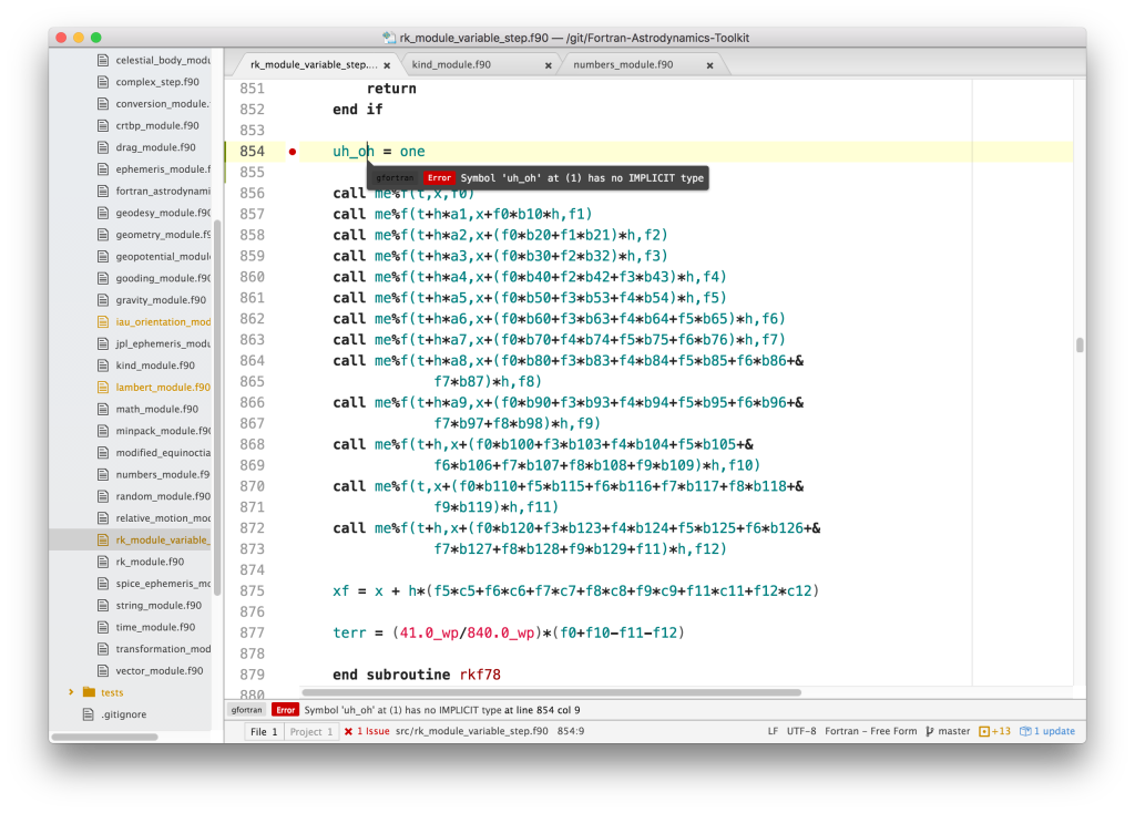
This newfangled Atom hipster text editor is really a nice editor for Fortran when you install these two plugins:
There are tons of other packages too. For example, indent-helper is a must, because every sane person knows that ='s and ::'s should always be aligned.
For many years, I've used TextWrangler by Bare Bones Software (which is the free version of their more powerful BBEdit). Just having the Fortran linter (see below) is enough to make me switch. I suppose with the right combination of plugins, I could use it as a full-fledged IDE, but I haven't really tried to do that yet.
Maybe one day @szaghi will write a FoBiS plugin for Atom. Unfortunately, I think he's totally committed to vi.
See also
Apr 05, 2016
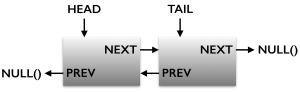
So, I want to have a basic linked list manager, written in modern Fortran (2003/2008). Of course, Fortran provides you with nothing like this out of the box, but it does provide the tools to create such a thing (within reason). Pointers (introduced in Fortran 90) allow for the creation of dynamic structures such as linked lists. In Fortran, you can do quite a lot without having to resort to pointers (say, compared to C, where you can't get away from them if you want to do anything nontrivial), but in this case, we need to use them. With the addition of unlimited polymorphic variables in Fortran 2003, we can now also create heterogeneous lists containing different types of variables, which is quite handy. There are some good Fortran linked-list implementations out there (see references below). But none seemed to do exactly what I wanted. Plus I wanted to learn about this stuff myself, so I went ahead and started from scratch. My requirements are that the code:
- Accept any data type from the caller. I don't want to force the caller to stuff their data into some standard form, or make them have to extend an abstract derived type to contain it.
- Accept data that may perhaps contain targets of pointers from other variables that are not in the list. This seems useful to me, but is an aspect that is missing from the implementations I have seen, as far as I can tell. If the data is being pointed to by something externally, doing a sourced allocation to create a copy is not acceptable, since the pointers will still be pointing to the original one and not the copy.
- Allow for the list to manage the destruction of the variable (deallocation of the pointer, finalization if it is present), or let the user handle it. Perhaps the list is being used to collocate and access some data, but if the list goes out of scope, the data is intended to remain.
- In general, limit the copying of data (some entries in the list may be very large and it is undesirable to make copies).
- Allow the key to be an integer or string (or maybe other variable types as well)
For lack of a better name, I've called the resultant library FLIST (it's on GitHub). It's really just an experiment at this point, but I think it does everything I need. The node data type used to construct the linked list is this:
type :: node
    private
    class(*),allocatable :: key
    class(*),pointer :: value => null()
    logical :: destroy_on_delete = .true.
    type(node),pointer :: next => null()
    type(node),pointer :: previous => null()
    contains
    private
    procedure :: destroy => destroy_node_data
end type node
The data in the node is a CLASS(*),POINTER variable (i.e, a pointer to an unlimited polymorphic variable). This will be associated to the data that is added to the list. Data can be added as a pointer (in which case no copying is performed), or added as a clone (where a new instance of the node data is instantiated and a copy of the input data is made). If the data is added as a pointer, the user can also optionally specify if the data is to be destroyed when the list is destroyed or goes out of scope (or if the item is deleted from the list).
The key is also an unlimited polymorphic variable (in the user-accessible API, keys are limited to integers, character strings, or extensions of an abstract key_class):
type,abstract,public :: key_class
    contains
    procedure(key_equal_func),deferred :: key_equal
    generic :: operator(==) => key_equal
end type key_class
The key types have to be limited, since there has to be a way to check for equality among keys (the abstract key_class has a deferred == operator that must be specified). The Fortran SELECT TYPE construct is used to resolve the polymorphic variables in order to check for equality among keys.
A simple example use case is shown below. Here we have some derived type gravity_model that is potentially very large, and is initialized by reading a data file. The subroutine takes as input a character array of file names to read, loads them, and appends the resultant models to the list_of_models.
subroutine add_some_models(files,list_of_models)

use linked_list_module
use gravity_model_module

implicit none

character(len=:),dimension(:),intent(in) :: files
type(list),intent(inout) :: list_of_models

integer :: i
type(gravity_model),pointer :: g

do i=1,size(files)
    allocate(g)
    call g%initialize(files(i))
    call list_of_models%add_pointer(files(i),g)
    nullify(g)
end do

end subroutine add_some_models
In this example, all the models are allocated in the subroutine, and then added as pointers to the list (the file name is used as the key). When list_of_models goes out of scope, the models will be deallocated (and finalized if gravity_model contains a finalizer). A model can be removed from the list (which will also trigger finalization) using the key, like so:
call list_of_models%remove('blah.dat')
More complex use cases are also possible (see the code for more details). As usual, the license is BSD, so if anybody else finds it useful, let me know.
See also
- T. Dunn, fortran-linked-list [GitHub]
- T. Degawa, LinkedList [GitHub]
- libAtoms/QUIP [GitHub]
- N. R. Papior, fdict [GitHub]
- C. MacMackin, FIAT [GitHub]
- J. R. Blevins, A Generic Linked List Implementation in Fortran 95, ACM Fortran Forum 28(3), 2–7, 2009.
Apr 03, 2016
Here is some C++ code (from actual NASA software):
aTilde[ 0] = aTilde[ 1] = aTilde[ 2] =
aTilde[ 3] = aTilde[ 4] = aTilde[ 5] =
aTilde[ 6] = aTilde[ 7] = aTilde[ 8] =
aTilde[ 9] = aTilde[10] = aTilde[11] =
aTilde[12] = aTilde[13] = aTilde[14] =
aTilde[15] = aTilde[16] = aTilde[17] =
aTilde[18] = aTilde[19] = aTilde[20] =
aTilde[21] = aTilde[22] = aTilde[23] =
aTilde[24] = aTilde[25] = aTilde[26] =
aTilde[27] = aTilde[28] = aTilde[29] =
aTilde[30] = aTilde[31] = aTilde[32] =
aTilde[33] = aTilde[34] = aTilde[35] = 0.0;
Here is the same code translated to Fortran:
😀
References
Mar 14, 2016
Fortran namelists are a quick and dirty way of reading and writing variables to and from a file. It is actually the only high-level file access feature built into the Fortran language, in the sense of being able to read and write a complex formatted file with one line of code. Nowadays, I would recommend against using this feature since the format is not really a standard and varies from compiler to compiler, and there aren't good parsers available for other languages (with the notable exception of Python). There are better configuration file formats available today such as JSON. However, namelists can still be encountered in legacy applications, and may still be useful to the lazy programmer.
One of the problems with namelists is that all the variables in the file have to correspond exactly in name, type, rank, and size to variables declared in your code. Syntax errors in the file are not easily detected and a failed read due to an unexpected variable will usually just return a non-zero status code that isn't really much help in diagnosing the problem.
However, there is a way to output the line where the failure occurred on a namelist read, which can be quite useful for debugging. Say your code is expecting a namelist containing three real variables a, b, and c. However, the file contains the unexpected variable d like so:
&my_namelist
 a = 1.0,
 b = 2.0,
 d = 3.0,
 c = 4.0
/
Now consider the following Fortran code to read it:
program namelist_test

use iso_fortran_env, wp => real64

implicit none

real(wp) :: a,b,c ! namelist variables
integer :: istat,iunit
character(len=1000) :: line

namelist /my_namelist/ a,b,c

open(newunit=iunit,file='my_namelist.nml',&
    status='OLD')

read(iunit, nml=my_namelist, iostat=istat)

if (istat/=0) then
    backspace(iunit)
    read(iunit,fmt='(A)') line
    write(error_unit,'(A)') &
        'Invalid line in namelist: '//trim(line)
end if

close(iunit)

end program namelist_test
The READ statement will fail with a non-zero istat code. Then we simply use the BACKSPACE function, which moves the file position back one record (the record where the read failed). Then we can simply read this line and print it. This code produces the following error message:
Invalid line in namelist: d = 3.0,
Feb 28, 2016
Some years ago, I needed a Fortran routine to do linear interpolation of a multidimensional (up to 6D) data set. Not wanting to reinvent the wheel, I ended up using a routine called FINT from CERNLIB (documentation here). It is written in Fortran 66, and has some hard-coded limits on the number of dimensions that can be used, but these are not fundamental to the algorithm. With a few minor changes, the routine can be used for interpolation of any number of dimensions. I present below a modern Fortran version that removes the limitations. Note that the original code is GPL licensed, thus so is this modification.
function fint(narg,arg,nent,ent,table)

use iso_fortran_env, only: wp => real64

implicit none

real(wp) :: fint
integer,intent(in) :: narg
integer,dimension(narg),intent(in) :: nent
real(wp),dimension(narg),intent(in) :: arg
real(wp),dimension(:),intent(in) :: ent
real(wp),dimension(:),intent(in) :: table

integer,dimension(2**narg) :: index
real(wp),dimension(2**narg) :: weight
logical :: mflag,rflag
real(wp) :: eta,h,x
integer :: i,ishift,istep,k,knots,lgfile,&
           lmax,lmin,loca,locb,locc,ndim

!some error checks:
if (size(ent)/=sum(nent)) &
    error stop 'size of ent is incorrect.'
if (size(table)/=product(nent)) &
    error stop 'size of table is incorrect.'
if (narg<1) &
    error stop 'invalid value of narg.'

lmax = 0
istep = 1
knots = 1
index(1) = 1
weight(1) = 1.0_wp

main: do i = 1 , narg
    x = arg(i)
    ndim = nent(i)
    loca = lmax
    lmin = lmax + 1
    lmax = lmax + ndim
    if ( ndim>2 ) then
        locb = lmax + 1
        do
            locc = (loca+locb)/2
            if ( x<ent(locc) ) then
                locb = locc
            else if ( x==ent(locc) ) then
                ishift = (locc-lmin)*istep
                do k = 1 , knots
                    index(k) = index(k) + ishift
                end do
                istep = istep*ndim
                cycle main
                else
                loca = locc
            end if
            if ( locb-loca<=1 ) exit
        end do
        loca = min(max(loca,lmin),lmax-1)
        ishift = (loca-lmin)*istep
        eta = (x-ent(loca))/(ent(loca+1)-ent(loca))
    else
        if ( ndim==1 ) cycle main
        h = x - ent(lmin)
        if ( h==0.0_wp ) then
            istep = istep*ndim
            cycle main
        end if
        ishift = istep
        if ( x-ent(lmin+1)==0.0_wp ) then
            do k = 1 , knots
                index(k) = index(k) + ishift
            end do
            istep = istep*ndim
            cycle main
        end if
        ishift = 0
        eta = h/(ent(lmin+1)-ent(lmin))
    end if
    do k = 1 , knots
        index(k) = index(k) + ishift
        index(k+knots) = index(k) + istep
        weight(k+knots) = weight(k)*eta
        weight(k) = weight(k) - weight(k+knots)
    end do
    knots = 2*knots
    istep = istep*ndim
end do main

fint = 0.0_wp
do k = 1 , knots
    i = index(k)
    fint = fint + weight(k)*table(i)
end do

end function fint
As I recall, I wrote wrappers to this function in order to be able to input the data in a more reasonable format. For example, for a five dimensional data set it is more natural to input the five rank-1 abscissa vectors and the rank-5 ordinate matrix. The disadvantage of this routine is that you have to stuff the ordinate matrix into a vector (as well as stuffing all the abscissa vectors into a single vector). This could also be an advantage in some cases, since Fortran arrays have a maximum rank. For Fortran 90, it was 7, while Fortran 2008 expanded this to 15 (the current Intel Fortran Compiler allows up to 31 as a non-standard extension). If you ever, for example, needed to interpolate 32-dimensional data (assuming you had enough RAM), you could do it with FINT without having to declare any rank-32 matrices. In any event, an example 5D wrapper for FINT is given here:
function fint_5d_wrapper(x,y,z,q,r,&
                         xvec,yvec,zvec,qvec,&
                         rvec,fmat) result(f)

use iso_fortran_env, only: wp => real64

implicit none

integer,parameter :: narg = 5

real(wp) :: f
real(wp),intent(in) :: x,y,z,q,r
real(wp),dimension(:),intent(in) :: xvec
real(wp),dimension(:),intent(in) :: yvec
real(wp),dimension(:),intent(in) :: zvec
real(wp),dimension(:),intent(in) :: qvec
real(wp),dimension(:),intent(in) :: rvec
real(wp),dimension(:,:,:,:,:),intent(in) :: fmat

integer,dimension(narg) :: nent

nent(1) = size(xvec)
nent(2) = size(yvec)
nent(3) = size(zvec)
nent(4) = size(qvec)
nent(5) = size(rvec)

f = fint(narg,[x,y,z,q,r],nent,&
    [xvec,yvec,zvec,qvec,rvec],&
    reshape(fmat,[product(nent)]))

end function fint_5d_wrapper
This works well enough, but note that it isn't very computationally efficient since we are creating temporary copies of the potentially large data arrays (including having to reshape a rank-5 matrix) every time we do an interpolation. While the logic of FINT is a bit hard to fathom, the actual equations are fairly simple (see here, for example). What we really need now is an object-oriented modern Fortran library for multidimensional linear interpolation. Stay tuned...
References
Feb 22, 2016
Intel has released version 16.0.2 of the Intel Fortran Compiler (which is part of Intel Parallel Studio XE 2016). It looks like mainly a bug-fix release. Microsoft Visual Studio 2015 Update 1 is now also officially supported.
References
Jan 31, 2016

*Thaddeus Vincenty (1920--2002) Image source: [IAG Newsletter](http://www.gfy.ku.dk/~iag/newslett/news7606.htm)*
There are two standard problems in geodesy:
- Direct geodetic problem -- Given a point on the Earth (latitude and longitude) and the direction (azimuth) and distance from that point to a second point, determine the latitude and longitude of that second point.
- Inverse geodetic problem -- Given two points on the Earth, determine the azimuth and distance between them.
Assuming the Earth is an oblate spheroid, both of these can be solved using the iterative algorithms by Thaddeus Vincenty [1]. Modern Fortran versions of Vincenty's algorithms can be found in the geodesy module of the Fortran Astrodynamics Toolkit [2].
The direct algorithm was listed in an earlier post. If we assume a WGS84 Earth ellipsoid (a=6378.137 km, f=1/298.257223563), an example direct calculation is:
$$
\begin{array}{rcll}
\phi_1 &= & 29.97^{\circ} & \mathrm{(Latitude ~of ~ first ~ point)}\\
\lambda_1 &= & -95.35^{\circ} & \mathrm{(Longitude ~of ~ first ~point)} \\
Az &= & 20^{\circ} & \mathrm{(Azimuth)}\\
s &= & 50~\mathrm{km} & \mathrm{(Distance)}
\end{array}
$$
The latitude and longitude of the second point is:
$$
\begin{array}{rcl}
\phi_2 &= & 30.393716^{\circ} \\
\lambda_2 &= & -95.172057^{\circ} \\
\end{array}
$$
The more complicated inverse algorithm is listed here (based on the USNGS code from [1]):
subroutine inverse(a, rf, b1, l1, b2, l2, faz, baz, s, it, sig, lam, kind)

    use, intrinsic :: iso_fortran_env, wp => real64

    implicit none

    real(wp), intent(in) :: a !! Equatorial semimajor axis
    real(wp), intent(in) :: rf !! reciprocal flattening (1/f)
    real(wp), intent(in) :: b1 !! latitude of point 1 (rad, positive north)
    real(wp), intent(in) :: l1 !! longitude of point 1 (rad, positive east)
    real(wp), intent(in) :: b2 !! latitude of point 2 (rad, positive north)
    real(wp), intent(in) :: l2 !! longitude of point 2 (rad, positive east)
    real(wp), intent(out) :: faz !! Forward azimuth (rad, clockwise from north)
    real(wp), intent(out) :: baz !! Back azimuth (rad, clockwise from north)
    real(wp), intent(out) :: s !! Ellipsoidal distance
    integer, intent(out) :: it !! iteration count
    real(wp), intent(out) :: sig !! spherical distance on auxiliary sphere
    real(wp), intent(out) :: lam !! longitude difference on auxiliary sphere
    integer, intent(out) :: kind !! solution flag: kind=1, long-line; kind=2, antipodal

    real(wp) :: beta1, beta2, biga, bigb, bige, bigf, boa, &
                c, cosal2, coslam, cossig, costm, costm2, &
                cosu1, cosu2, d, dsig, ep2, l, prev, sinal, &
                sinlam, sinsig, sinu1, sinu2, tem1, tem2, &
                temp, test, z

    real(wp), parameter :: pi = acos(-1.0_wp)
    real(wp), parameter :: two_pi = 2.0_wp*pi
    real(wp), parameter :: tol = 1.0e-14_wp !! convergence tolerance
    real(wp), parameter :: eps = 1.0e-15_wp !! tolerance for zero

    boa = 1.0_wp - 1.0_wp/rf

    beta1 = atan(boa*tan(b1))
    sinu1 = sin(beta1)
    cosu1 = cos(beta1)
    beta2 = atan(boa*tan(b2))
    sinu2 = sin(beta2)
    cosu2 = cos(beta2)

    l = l2 - l1
    if (l > pi) l = l - two_pi
    if (l < -pi) l = l + two_pi
    prev = l
    test = l
    it = 0
    kind = 1
    lam = l

    longline: do ! long-line loop (kind=1)

        sinlam = sin(lam)
        coslam = cos(lam)
        temp = cosu1*sinu2 - sinu1*cosu2*coslam
        sinsig = sqrt((cosu2*sinlam)**2 + temp**2)
        cossig = sinu1*sinu2 + cosu1*cosu2*coslam
        sig = atan2(sinsig, cossig)
        if (abs(sinsig) < eps) then
            sinal = cosu1*cosu2*sinlam/sign(eps, sinsig)
        else
            sinal = cosu1*cosu2*sinlam/sinsig
        end if
        cosal2 = -sinal**2 + 1.0_wp
        if (abs(cosal2) < eps) then
            costm = -2.0_wp*(sinu1*sinu2/sign(eps, &
                                              cosal2)) + cossig
        else
            costm = -2.0_wp*(sinu1*sinu2/cosal2) + &
                    cossig
        end if
        costm2 = costm*costm
        c = ((-3.0_wp*cosal2 + 4.0_wp)/rf + 4.0_wp)* &
            cosal2/rf/16.0_wp

        antipodal: do ! antipodal loop (kind=2)

            it = it + 1
            d = (((2.0_wp*costm2 - 1.0_wp)*cossig*c + &
                  costm)*sinsig*c + sig)*(1.0_wp - c)/rf
            if (kind == 1) then
                lam = l + d*sinal
                if (abs(lam - test) >= tol) then
                    if (abs(lam) > pi) then
                        kind = 2
                        lam = pi
                        if (l < 0.0_wp) lam = -lam
                        sinal = 0.0_wp
                        cosal2 = 1.0_wp
                        test = 2.0_wp
                        prev = test
                        sig = pi - abs(atan(sinu1/cosu1) + &
                                    atan(sinu2/cosu2))
                        sinsig = sin(sig)
                        cossig = cos(sig)
                        c = ((-3.0_wp*cosal2 + 4.0_wp)/rf + &
                            4.0_wp)*cosal2/rf/16.0_wp
                        if (abs(sinal - prev) < tol) exit longline
                        if (abs(cosal2) < eps) then
                            costm = -2.0_wp*(sinu1*sinu2/ &
                                            sign(eps, cosal2)) + cossig
                        else
                            costm = -2.0_wp*(sinu1*sinu2/cosal2) + &
                                    cossig
                        end if
                        costm2 = costm*costm
                        cycle antipodal
                    end if
                    if (((lam - test)*(test - prev)) < 0.0_wp .and. it > 5) &
                        lam = (2.0_wp*lam + 3.0_wp*test + prev)/6.0_wp
                    prev = test
                    test = lam
                    cycle longline
                end if
            else
                sinal = (lam - l)/d
                if (((sinal - test)*(test - prev)) < 0.0_wp .and. it > 5) &
                    sinal = (2.0_wp*sinal + 3.0_wp*test + prev)/6.0_wp
                prev = test
                test = sinal
                cosal2 = -sinal**2 + 1.0_wp
                sinlam = sinal*sinsig/(cosu1*cosu2)
                coslam = -sqrt(abs(-sinlam**2 + 1.0_wp))
                lam = atan2(sinlam, coslam)
                temp = cosu1*sinu2 - sinu1*cosu2*coslam
                sinsig = sqrt((cosu2*sinlam)**2 + temp**2)
                cossig = sinu1*sinu2 + cosu1*cosu2*coslam
                sig = atan2(sinsig, cossig)
                c = ((-3.0_wp*cosal2 + 4.0_wp)/rf + 4.0_wp)* &
                    cosal2/rf/16.0_wp
                if (abs(sinal - prev) >= tol) then
                if (abs(cosal2) < eps) then
                    costm = -2.0_wp*(sinu1*sinu2/ &
                                     sign(eps, cosal2)) + cossig
                else
                    costm = -2.0_wp*(sinu1*sinu2/cosal2) + &
                            cossig
                end if
                costm2 = costm*costm
                cycle antipodal
                end if
            end if

            exit longline

        end do antipodal

    end do longline

    if (kind == 2) then ! antipodal
        faz = sinal/cosu1
        baz = sqrt(-faz**2 + 1.0_wp)
        if (temp < 0.0_wp) baz = -baz
        faz = atan2(faz, baz)
        tem1 = -sinal
        tem2 = sinu1*sinsig - cosu1*cossig*baz
        baz = atan2(tem1, tem2)
    else ! long-line
        tem1 = cosu2*sinlam
        tem2 = cosu1*sinu2 - sinu1*cosu2*coslam
        faz = atan2(tem1, tem2)
        tem1 = -cosu1*sinlam
        tem2 = sinu1*cosu2 - cosu1*sinu2*coslam
        baz = atan2(tem1, tem2)
    end if

    if (faz < 0.0_wp) faz = faz + two_pi
    if (baz < 0.0_wp) baz = baz + two_pi
    ep2 = 1.0_wp/(boa*boa) - 1.0_wp
    bige = sqrt(1.0_wp + ep2*cosal2)
    bigf = (bige - 1.0_wp)/(bige + 1.0_wp)
    biga = (1.0_wp + bigf*bigf/4.0_wp)/(1.0_wp - bigf)
    bigb = bigf*(1.0_wp - 0.375_wp*bigf*bigf)
    z = bigb/6.0_wp*costm*(-3.0_wp + 4.0_wp* &
                           sinsig**2)*(-3.0_wp + 4.0_wp*costm2)
    dsig = bigb*sinsig*(costm + bigb/4.0_wp* &
                        (cossig*(-1.0_wp + 2.0_wp*costm2) - z))
    s = (boa*a)*biga*(sig - dsig)

end subroutine inverse
For the same ellipsoid, an example inverse calculation is:
$$
\begin{array}{rcll}
\phi_1 &= & 29.97^{\circ} & \mathrm{(Latitude ~of ~ first ~ point)}\\
\lambda_1 &= & -95.35^{\circ} & \mathrm{(Longitude ~of ~ first ~point)} \\
\phi_2 &= & 40.77^{\circ} & \mathrm{(Latitude ~of ~ second ~ point)}\\
\lambda_2 &= & -73.98^{\circ} & \mathrm{(Longitude ~of ~ second ~point)}
\end{array}
$$
The azimuth and distance from the first to the second point is:
$$
\begin{array}{rcl}
Az &= & 52.400056^{\circ} & \mathrm{(Azimuth)}\\
s &= & 2272.497~\mathrm{km} & \mathrm{(Distance)}
\end{array}
$$
References
